8.5 Unit-Root Nonstationarity and Cointegration

When modeling several unit-root nonstationary time series jointly, one may encounter the case of cointegration. Consider the bivariate ARMA(1,1) model

8.31

where the covariance matrix of the shock is positive definite. This is not a weakly stationary model because the two eigenvalues of the AR coefficient matrix are 0 and 1. Figure 8.10 shows the time plots of a simulated series of the model with 200 data points and = , whereas Figure 8.11 shows the sample autocorrelations of the two component series xit. It is easy to see that the two series have high autocorrelations and exhibit features of unit-root nonstationarity. The two marginal models of are indeed unit-root nonstationary. Rewrite the model as

Premultiplying the above equation by

we obtain the result

Therefore, each component xit of the model is unit-root nonstationary and follows an ARIMA(0,1,1) model.

Figure 8.10 Time plots of simulated series based on model (8.31) with identity covariance matrix for shocks.

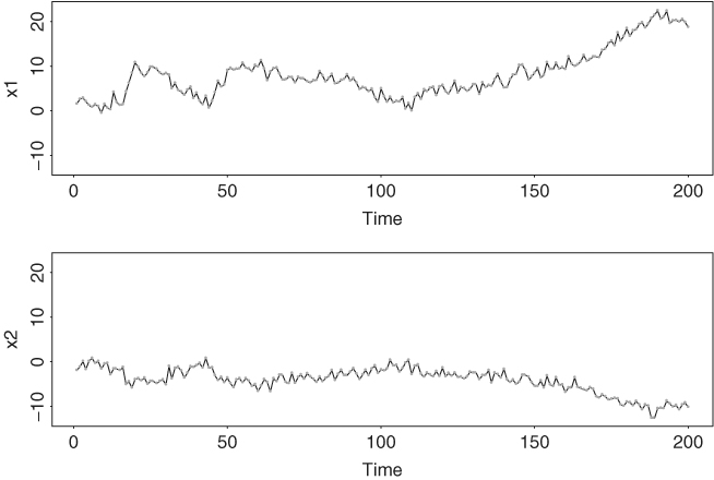
Figure 8.11 Sample autocorrelation functions of two simulated component series. There are 200 observations, and model is given by Eq. (8.34) with identity covariance matrix for shocks.

However, we can consider a linear transformation by defining

The VARMA model of the transformed series can be obtained as follows:

Thus, the model for is

8.32

From the prior model, we see that (a) y1t and y2t are uncoupled series with concurrent correlation equal to that between the shocks b1t and b2t, (b) y1t follows a univariate ARIMA(0,1,1) model, and (c) y2t is a white noise series (i.e., y2t = b2t). In particular, the model in Eq. (8.32) shows that there is only a single unit root in the system. Consequently, the unit roots of x1t and x2t are introduced by the unit root of y1t. In the literature, y1t is referred to as the common trend of x1t and x2t.

The phenomenon that both x1t and x2t are unit-root nonstationary, but there is only a single unit root in the vector series, is referred to as cointegration in the econometric and time series literature. Another way to define cointegration is to focus on linear transformations of unit-root nonstationary series. For the simulated example of model (8.31), the transformation shows that the linear combination y2t = 0.5x1t + x2t does not have a unit root. Consequently, x1t and x2t are cointegrated if (a) both of them are unit-root nonstationary, and (b) they have a linear combination that is unit-root stationary.

Generally speaking, for a k-dimensional unit-root nonstationary time series, cointegration exists if there are less than k unit roots in the system. Let h be the number of unit roots in the k-dimensional series . Cointegration exists if 0 < h < k, and the quantity k − h is called the number of cointegrating factors. Alternatively, the number of cointegrating factors is the number of different linear combinations that are unit-root stationary. The linear combinations are called the cointegrating vectors. For the prior simulated example, so that (0.5, 1)′ is a cointegrating vector for the system. For more discussions on cointegration and cointegration tests, see Box and Tiao (1977), Engle and Granger (1987), Stock and Watson (1988), and Johansen (1988). We discuss cointegrated VAR models in Section 8.6.

The concept of cointegration is interesting and has attracted a lot of attention in the literature. However, there are difficulties in testing for cointegration in a real application. The main source of difficulties is that cointegration tests overlook the scaling effects of the component series. Interested readers are referred to Cochrane (1988) and Tiao, Tsay, and Wang (1993) for further discussion.

While I have some misgivings on the practical value of cointegration tests, the idea of cointegration is highly relevant in financial study. For example, consider the stock of Finnish Nokia Corporation. Its price on the Helsinki Stock Market must move in unison with the price of its American Depositary Receipts on the New York Stock Exchange; otherwise there exists some arbitrage opportunity for investors. If the stock price has a unit root, then the two price series must be cointegrated. In practice, such a cointegration can exist after adjusting for transaction costs and exchange rate risk. We discuss issues like this later in Section 8.7.

8.5.1 An Error Correction Form

Because there are more unit-root nonstationary components than the number of unit roots in a cointegrated system, differencing individual components to achieve stationarity results in overdifferencing. Overdifferencing leads to the problem of unit roots in the MA matrix polynomial, which in turn may encounter difficulties in parameter estimation. If the MA matrix polynomial contains unit roots, the vector time series is said to be noninvertible.

Engle and Granger (1987) discuss an error correction representation for a cointegrated system that overcomes the difficulty of estimating noninvertible VARMA models. Consider the cointegrated system in Eq. (8.31). Let be the differenced series. Subtracting from both sides of the equation, we obtain a model for as

This is a stationary model because both and = y2t are unit-root stationary. Because is used on the right-hand side of the previous equation, the MA matrix polynomial is the same as before and, hence, the model does not encounter the problem of noninvertibility. Such a formulation is referred to as an error correction model for , and it can be extended to the general cointegrated VARMA model. For a cointegrated VARMA(p, q) model with m cointegrating factors (m < k), an error correction representation is

8.33

where and are k × m full-rank matrices. The AR coefficient matrices are functions of the original coefficient matrices . Specifically, we have

8.34

These results can be obtained by equating coefficient matrices of the AR matrix polynomials. The time series is unit-root stationary, and the columns of are the cointegrating vectors of .

Existence of the stationary series in the error correction representation (8.33) is natural. It can be regarded as a “compensation” term for the overdifferenced system . The stationarity of can be justified as follows. The theory of unit-root time series shows that the sample correlation coefficient between a unit-root nonstationary series and a stationary series converges to zero as the sample size goes to infinity; see Tsay and Tiao (1990) and the references therein. In an error correction representation, is unit-root nonstationary, but is stationary. Therefore, the only way that can relate meaningfully to is through a stationary series .