
Pairs trading is a market-neutral trading strategy. There are several versions of pairs trading in the equity markets. In this section, we focus on the statistical arbitrage pairs trading, which makes use of the ideas of cointegration and error correction model discussed in the chapter. Our discussion will be brief. For more information concerning pairs trading and statistical arbitrage, see Vidyamurthy (2004) and Pole (2007).
The general theme for trading in the equity markets is to buy undervalued stocks and sell overvalued ones. However, the true price of a stock is hard to assess. Pairs trading attempts to resolve this difficulty using the idea of relative pricing. Based on the arbitrage pricing theory (APT) in finance, if two stocks have similar characteristics, then the prices of both stocks must be more or less the same. If the prices differ, then it is likely that one of the stocks is overpriced and the other underpriced. Pairs trading involves selling the higher priced stock and buying the lower priced stock with the hope that the mispricing will correct itself in the future. Note that the true prices of the two stocks are not important. The observed prices may be wrong. What is important is that the observed prices be the same. The gap (properly scaled) between the two observed prices is called the spread. For pairs trading, the greater the spread, the larger the magnitude of mispricing and the greater the profit potential. Before discussing a trading strategy, we first introduce the theoretical framework.
8.8.1 Theoretical Framework
Consider two stocks. Let Pit be the observed price of stock i at time t and pit = ln(Pit) be the corresponding log price. As mentioned in earlier chapters, it is reasonable to assume that pit is unit-root nonstationary and follows a random-walk model; that is, pit = pi, t−1 + rit, where {rit} is the return and forms a sequence of uncorrelated innovations. If the two stocks have similar risk factors, then they should have similar returns based on APT. Therefore, p1t and p2t are likely to be driven by a common component and are cointegrated. In other words, there exists a linear combination wt = p1t − γp2t, which is unit-root stationary and, hence, mean reverting. The two price series {p1t} and {p2t} thus assume an error correction form
where μw = E(wt) denotes the mean of wt. The four parameters γ, μw, α1, and α2 can be estimated, for instance, by the maximum-likelihood or least-squares methods; see Section 8.6.2. We refer to the stationary series wt as the spread between the two log stock prices.
The left-hand side of Eq. (8.45) consists the log returns of the two stocks. The equation says that the returns depend on wt−1, which is the stationary. Specifically, wt−1 − μw denotes the deviation from the log-run equilibrium between the two stocks. Equation (8.45) shows that, for cointegrated stocks, the returns depend on the past deviation from equilibrium. The coefficients α1 and α2 show the effect of past deviation on the returns r1t and r2t, respectively. In practice, α1 and α2 should have opposite signs, indicating reversion to the equilibrium.
Next, consider a portfolio with long one share of stock 1 and short γ shares of stock 2. The return of the portfolio for a given time period i is
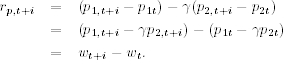
Therefore, the return rp, t+i of the portfolio is the increment of the spread in the time period. As expected, the return of the portfolio does not depend on the mean of wt.
8.8.2 Trading Strategy
The idea behind a pairs-trading strategy is to trade on the oscillations about the equilibrium value of the spread. The oscillations in spread occur because the spread is mean reverting. Since the equilibrium value is the mean of wt, that is, μw, we can put on a trade when wt deviates substantially from its mean and unwind the trade when the equilibrium is restored. In practice, how big the deviation needs to be in order for the trading to be profitable depends on several factors. Trading costs, marginal interest rates, and bid–ask spreads of the two stocks are three obvious factors. Mathematically, let η be the cost involved in carrying out a pairs trading. Let Δ be a target deviation of wt from its mean μw for pairs trading. Then, conditioned on 2Δ > η, a simple trading strategy is as follows:
- Buy a share of stock 1 and short γ shares of stock 2 at time t if wt = p1t − γp2t = μw − Δ.
- Unwind the position at time t + i (i > 0) if wt+i = p1, i+i − γp2, t+i = μw + Δ.
One can identify the time point t so long as Δ is not too large compared with the standard deviation of wt. The time point t + i will occur because of the mean reverting of the spread series. In this particular instance, the return of the portfolio wt+i − wt = 2Δ and the net profit of the trade is 2Δ − η > 0.
DiscussionThe aforementioned trading strategy is just one of many possibilities. For instance, if Δ > η, one can unwind the position when wt+i = μw. The net profit of the pairs trading then is Δ − η > 0. This may result in more transactions and trading costs, but it shortens the holding period of the portfolio. If Δ is negative, then one can short one share of stock 1 and buy γ shares of stock 2 to make a net profit − 2Δ − η. The quantity η is the threshold for trading and is likely to depend on several factors such as transaction fees and bid–ask spreads of the two stocks.
8.8.3 Simple Illustration
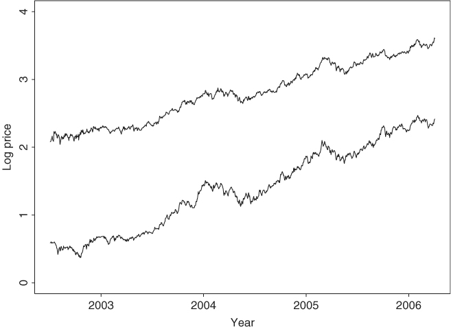
To demonstrate pairs trading, we consider two stocks traded on the New York Stock Exchange. The two companies are the Billiton Ltd. of Australia and the Vale S.A. of Brazil with stock symbols BHP and VALE, respectively. BHP of Australia is a natural resources company with business in Australia, the Americans, and Southern Africa. Vale of Brazil is a worldwide metals and mining company. Thus, both multinational companies belong to the natural resources industry and encounter similar risk factors. The daily prices of the two stocks were downloaded from Yahoo Finance, and we employ adjusted closing prices from July 1, 2002, to March 31, 2006, in our study.
Figure 8.17 shows the time plots of the daily log prices of the two stocks (adjusted closing prices). The upper plot is for the BHP stock. From the plots, the prices of the two stocks exhibit certain characteristics of comovement. Let p1t and p2t be the daily log closing prices of BHP and VALE, respectively. We analyze the series using both the least-squares and maximum-likelihood methods.
Figure 8.17 Daily log (adjusted) closing prices of BHP and VALE stocks from July 1, 2002, to March 31, 2006. Upper plot is for BHP stock.
8.8.3.1 Least-Squares Estimation
A simple way to verify that the two stocks are suitable for pairs trading is to check the cointegration of their log stock prices. To this end, we consider the simple linear regression p1t = β0 + β1p2t + wt, where wt denotes the residual series. For the BHP and VALE stocks, we have
![]()
Figure 8.18(a) shows the time plot of the residual series ![]() t. The plot shows that the residual series has certain characteristics of a stationary time series. In particular, it has mean zero and fluctuates around its mean within a fixed range. Figure 8.18(b) gives the sample ACF of
t. The plot shows that the residual series has certain characteristics of a stationary time series. In particular, it has mean zero and fluctuates around its mean within a fixed range. Figure 8.18(b) gives the sample ACF of ![]() t. The ACFs decay exponentially, supporting that
t. The ACFs decay exponentially, supporting that ![]() t is indeed stationary. To further confirm the stationarity assertion, we fit an AR(2) model to
t is indeed stationary. To further confirm the stationarity assertion, we fit an AR(2) model to ![]() t and obtain
t and obtain
![]()
Following the discussion of Chapter 2, we can obtain the two characteristic roots of the fitted AR(2) model. Indeed, the model can be rewritten as (1 − 0.935B)(1 − 0.130B)![]() t = at. Hence,
t = at. Hence, ![]() t is stationary. Finally, we conduct an augmented Dickey–Fuller unit-root test on
t is stationary. Finally, we conduct an augmented Dickey–Fuller unit-root test on ![]() t using an AR(2) model and find that the test statistic is − 6.04 with a p value of 0.01. The unit-root hypothesis is clearly rejected.
t using an AR(2) model and find that the test statistic is − 6.04 with a p value of 0.01. The unit-root hypothesis is clearly rejected.
Figure 8.18 Results of least-squares estimation: (a) Time plot of the estimated spread between BHP and VALE daily log stock prices. (b) Sample autocorrelation functions of estimated spread.

8.8.3.2 Maximum-Likelihood Estimation
A formal approach to verify the cointegration of the two log stock prices is to perform a cointegration test. Let ![]() . Using information criteria, a VAR(1) model is specified for
. Using information criteria, a VAR(1) model is specified for ![]() . We then conduct cointegration tests with restricted and unrestricted constant. Both tests give similar results so that we only report the results for the case of restricted constant.
. We then conduct cointegration tests with restricted and unrestricted constant. Both tests give similar results so that we only report the results for the case of restricted constant.
> coint2=coint(xx,trend=“rc”)
> coint2
coint(Y = xt, trend = “rc”)
Trend Specification:
H1*(r): Restricted constant
Trace tests signif. at the 5% level are flagged by ‘ +’.
Trace tests signif. at the 1% level are flagged by ‘++’.
Max Eigenvalue tests signif. at the 5% level are
flagged by ‘ *’.
Max Eigenvalue tests signif. at the 1% level are
flagged by ‘**’.
Tests for Cointegration Rank:
Eigenvalue TraceSt 95%-CV 99%-CV Max-St 95%-CV 99%-CV
H(0)++** 0.0415 47.7400 19.960 24.600 39.965 15.670 20.200
H(1) 0.0082 7.7748 9.240 12.970 7.774 9.240 12.970
The test confirms that ![]() is cointegrated. Next, we perform the maximum-likelihood estimation of the error correction model. The results are given below:
is cointegrated. Next, we perform the maximum-likelihood estimation of the error correction model. The results are given below:
> n3=VECM(coint2)
> summary(n3)
VECM(test = coint2)
Cointegrating Vectors:
coint.1
1.0000
vale −0.7177
(std.err) 0.0112
(t.stat) −64.0913
Intercept* −1.8144
(std.err) 0.0169
(t.stat) −107.0430
VECM Coefficients:
bhp vale
coint.1 −0.0671 0.0263
(std.err) 0.0145 0.0168
(t.stat) −4.6462 1.5659
bhp.lag1 −0.1119 0.0659
(std.err) 0.0366 0.0425
(t.stat) −3.0596 1.5516
vale.lag1 0.0732 0.0445
(std.err) 0.0320 0.0371
(t.stat) 2.2920 1.1986
Regression Diagnostics:
bhp vale
R-squared 0.0370 0.0104
Adj. R-squared 0.0350 0.0083
Resid. Scale 0.0193 0.0224
Based on the estimation result, we have the model
![]()
where the estimated standard errors of ait are 0.019 and 0.022, respectively. In addition, the spread series is wt = p1t − 0.718p2t, which is stationary with mean 1.81. Clearly, the result is very close to that of the least-squares estimation. In particular, the γ parameter for the pairs trading is ![]() . Also, as expected, α1 is negative whereas α2 is positive.
. Also, as expected, α1 is negative whereas α2 is positive.
8.8.3.3 Trading Strategy
Since the standard error of the spread series wt is 0.044, we can select Δ = 0.045, which is slightly greater than one standard error of wt, for pairs trading. This choice of Δ ensures that the probability for the spread wt to deviate Δ away from its mean is not small. In fact, under the normality assumption, the probability is about 30%. Figure 8.19 shows the time plot of the spread series wt of the fitted error correction model. Three horizontal lines are imposed on the plot. They are μw, μw + 0.045, and μw − 0.045 with the latter two serving as boundaries for pairs trading. Since wt varies from the lower boundary to the upper one (or from the upper boundary to the lower one) several times, there are many pairs-trading opportunities. From the discussion of Section 8.8.2, the log return of each pairs trading is 2Δ = 0.09, which is not small. A more realistic demonstration is to implement the trading in a out-of-sample period. However, the example shows that pairs trading is feasible.
Figure 8.19 Time plot of fitted spread series between daily log prices of BHP and VALE stocks. Three horizontal lines denotes μw, μw + 0.045, and μw − 0.045 with μw = E(wt).

Finally, an important question in pairs trading is to identify the cointegrated pairs of stocks. There are some procedures available in the literature. It seems reasonable to consider pairs of stocks that have similar risk factors. In other words, one should make use of finance theory to guide the selection.
8.8.3.4 R Demonstration
The following output has been edited:
> library(urca)
> help(ca.jo)
> da=read.table(“d-bhp0206.txt”,header=T)
> da1=read.table(“d-vale0206.txt”,header=T)
> bhp=log(da[,9])
> vale=log(da1[,9])
> m1=lm(bhp˜vale)
> summary(m1)
Call:
lm(formula = bhp ˜ vale)
Coefficients:
Estimate Std. Error t value Pr(>|t|)
(Intercept) 1.822648 0.003662 497.7 >2e−16 ***
vale 0.716664 0.002354 304.4 >2e−16 ***
---
Residual standard error: 0.04421 on 944 degrees of freedom
Multiple R-squared: 0.9899, Adjusted R-squared: 0.9899
F-statistic: 9.266e+04 on 1 and 944 DF, p-value: < 2.2e−16
> wt=m1$residuals
> m3=arima(wt,order=c(2,0,0),include.mean=F)
> m3
Call:
arima(x = wt, order = c(2, 0, 0), include.mean = F)
Coefficients:
ar1 ar2
0.8051 0.1219
s.e. 0.0322 0.0325
sigmaˆ2 estimated as 0.0003326: log likelihood=2444.76
> p1=c(1,-m3$coef)
> x=polyroot(p1)
> x
[1] 1.069100+0i −7.675365-0i
> 1/Mod(x)
[1] 0.9353661 0.1302870
> xt=cbind(bhp,vale)
> mm=ar(xt)
> mm$order
[1] 2
> cot=ca.jo(xt,ecdet=‘const’,type=‘trace’,K=2,
spec=‘transitory’)
> summary(cot)
######################
# Johansen-Procedure #
######################
Test type: trace statistic, without linear trend and
constant in cointegration
Eigenvalues (lambda):
[1] 4.148282e−02 8.206470e−03 −4.610389e−18
Values of teststatistic and critical values of test:
test 10pct 5pct 1pct
r <= 1 | 7.78 7.52 9.24 12.97
r = 0 | 47.77 17.85 19.96 24.60
Eigenvectors, normalised to first column:
(These are the cointegration relations)
bhp.l1 vale.l1 constant
bhp.l1 1.000000 1.0000000 1.000000
vale.l1 −0.717704 −0.7327542 2.047274
constant −1.828460 −1.5411890 −5.712629
Weights W:
(This is the loading matrix)
bhp.l1 vale.l1 constant
bhp.d −0.06731196 0.004568985 9.341093e−18
vale.d 0.02545606 0.007541565 1.015639e−18
> co1=ca.jo(xt,ecdet=“const”,type=‘eigen’,K=2,
spec=‘transitory’)
> summary(co1)
######################
# Johansen-Procedure #
######################
Test type: maximal eigenvalue statistic (lambda max), without
linear trend and constant in cointegration
Eigenvalues (lambda):
[1] 4.148282e−02 8.206470e−03 −4.610389e−18
Values of teststatistic and critical values of test:
test 10pct 5pct 1pct
r <= 1 | 7.78 7.52 9.24 12.97
r = 0 | 40.00 13.75 15.67 20.20
Eigenvectors, normalised to first column:
(These are the cointegration relations)
bhp.l1 vale.l1 constant
bhp.l1 1.000000 1.0000000 1.000000
vale.l1 −0.717704 −0.7327542 2.047274
constant −1.828460 −1.5411890 −5.712629
Weights W:
(This is the loading matrix)
bhp.l1 vale.l1 constant
bhp.d −0.06731196 0.004568985 9.341093e−18
vale.d 0.02545606 0.007541565 1.015639e−18