
R is a free software available from http://www.r-project.org. One can click CRAN on its Web page to select a nearby CRAN Mirror to download and install the software and selected packages. For financial time series analysis, the Rmetrics of Diethelm Wuertz and his associates have produced many useful packages, including fBasics, timeSeries, fGarch, etc. We use many functions of these packages in this book. Further information concerning installing R and the commands used can be found either on the Web page of this book or on the author's teaching Web page.
R and S-Plus are objective-oriented software. They enable users to create many objects. For instance, one can use the command ts to create a time series object. Treating time series data as a time series object in R has some advantages, but it requires some learning to get used to it. It is, however, not necessary to create a time series object in R to perform the analyses discussed in this book. As an illustration, consider the monthly simple returns to the General Motors stock from January 1975 to December 2008; see Exercise 1.2. The data have 408 observations. The following R commands are used to illustrate the points:
> da=read.table(“m-gm3dx7508.txt”,header=T) % Load data
> gm=da[,2] % Column 2 contains GM stock returns
> gm1=ts(gm,frequency=12,start=c(1975,1))
% Creates a ts object.
> par(mfcol=c(2,1)) % Put two plots on a page.
> plot(gm,type=‘l’)
> plot(gm1,type=‘l’)
> acf(gm,lag=24)
> acf(gm1,lag=24)
In the ts command, frequency = 12 says that the time unit is year and there are 12 equally spaced observations in each time unit, and start = c(1975,1) means the starting time is January 1975. Frequency and start are the two basic arguments needed in R to create a time series object. For further details, please use help(ts) in R to obtain details of the command. Here gm1 is a time series object in R, but gm is not. Figures 1.7 and 1.8 show, respectively, the time plot and autocorrelation function (ACF) of the returns of GM stock. In each figure, the upper plot is produced without using time series object, whereas the lower plot is produced by a time series object. The upper and lower plots are identical except for the horizontal label. For the time plot, the time series object uses calendar time to label the x axis, which is preferred. On the other hand, for the ACF plot, the time series object uses fractions of time unit in the label, not the commonly used time lags.
Figure 1.6 Time plot of daily exchange rate between U.S. dollar and Japanese yen from January 4, 2000, to March 27, 2009: (a) exchange rate and (b) changes in exchange rate.
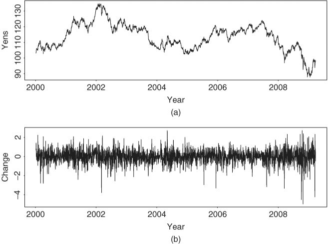
Figure 1.7 Time plots of monthly simple returns to General Motors stock from January 1975 to December 2008: (a) and (b) are without and with time series object, respectively.
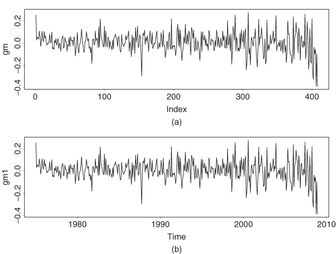
Figure 1.8 Sample ACFs of the monthly simple returns to General Motors stock from January 1975 to December 2008: (a) and (b) are without and with time series object, respectively.

Exercises
1.1 Consider the daily stock returns of American Express (AXP), Caterpillar (CAT), and Starbucks (SBUX) from January 1999 to December 2008. The data are simple returns given in the file d-3stocks9908.txt (date, axp, cat, sbux).
a. Express the simple returns in percentages. Compute the sample mean, standard deviation, skewness, excess kurtosis, minimum, and maximum of the percentage simple returns.
b. Transform the simple returns to log returns.
c. Express the log returns in percentages. Compute the sample mean, standard deviation, skewness, excess kurtosis, minimum, and maximum of the percentage log returns.
d. Test the null hypothesis that the mean of the log returns of each stock is zero. That is, perform three separate tests. Use 5% significance level to draw your conclusion.
1.2 Answer the same questions as in Exercise 1.1 but using monthly stock returns for General Motors (GM), CRSP value-weighted index (VW), CRSP equal-weighted index (EW), and S&P composite index from January 1975 to December 2008. The returns of the indexes include dividend distributions. Data file is m-gm3dx7508.txt (date, gm, vw, ew, sp).
1.3 Consider the monthly stock returns of S&P composite index from January 1975 to December 2008 in Exercise 1.2. Answer the following questions:
a. What is the average annual log return over the data span?
b. Assume that there were no transaction costs. If one invested $1.00 on the S&P composite index at the beginning of 1975, what was the value of the investment at the end of 2008?
1.4 Consider the daily log returns of American Express stock from January 1999 to December 2008 as in Exercise 1.1. Use the 5% significance level to perform the following tests: (a) Test the null hypothesis that the skewness measure of the returns is zero. (b) Test the null hypothesis that the excess kurtosis of the returns is zero.
1.5 Daily foreign exchange rates (spot rates) can be obtained from the Federal Reserve Bank in Chicago. The data are the noon buying rates in New York City certified by the Federal Reserve Bank of New York. Consider the exchange rates between the U.S. dollar and the Canadian dollar, euro, U.K. pound, and the Japanese yen from January 4, 2000, to March 27, 2009. The data are also on the Web. (a) Compute the daily log return of each exchange rate. (b) Compute the sample mean, standard deviation, skewness, excess kurtosis, minimum, and maximum of the log returns of each exchange rate. (c) Discuss the empirical characteristics of the log returns of exchange rates. (d) Obtain a density plot of the daily long returns of dollar–euro exchange rate.
Campbell, J. Y., Lo, A. W., and MacKinlay, A. C. (1997). The Econometrics of Financial Markets. Princeton University Press, Princeton, NJ.
Jarque, C. M. and Bera, A. K. (1987). A test of normality of observations and regression residuals. International Statistical Review 55: 163–172.
Sharpe, W. (1964). Capital asset prices: A theory of market equilibrium under conditions of risk. Journal of Finance 19: 425–442.
Snedecor, G. W. and Cochran, W. G. (1980). Statistical Methods, 7th ed. Iowa State University Press, Ames, IA.