2.9 Regression Models with Time Series Errors

In many applications, the relationship between two time series is of major interest. An obvious example is the market model in finance that relates the excess return of an individual stock to that of a market index. The term structure of interest rates is another example in which the time evolution of the relationship between interest rates with different maturities is investigated. These examples lead naturally to the consideration of a linear regression in the form

2.43

where yt and xt are two time series and et denotes the error term. The least-squares (LS) method is often used to estimate model (2.43). If {et} is a white noise series, then the LS method produces consistent estimates. In practice, however, it is common to see that the error term et is serially correlated. In this case, we have a regression model with time series errors, and the LS estimates of α and β may not be consistent.

A regression model with time series errors is widely applicable in economics and finance, but it is one of the most commonly misused econometric models because the serial dependence in et is often overlooked. It pays to study the model carefully.

We introduce the model by considering the relationship between two U.S. weekly interest rate series:

Both series have 2467 observations from January 5, 1962, to April 10, 2009, and are measured in percentages. The series are obtained from the Federal Reserve Bank of St Louis. Strictly speaking, we should model the two interest series jointly using multivariate time series analysis in Chapter 8. However, for simplicity, we focus here on regression-type analysis and ignore the issue of simultaneity.

Figure 2.17 shows the time plots of the two interest rates with a solid line denoting the 1-year rate and a dashed line the 3-year rate. Figure 2.18(a) plots r1t versus r3t, indicating that, as expected, the two interest rates are highly correlated. A naive way to describe the relationship between the two interest rates is to use the simple model r3t = α + βr1t + et. This results in a fitted model

2.44

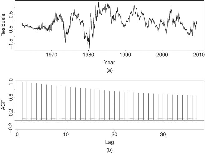
with R2 = 96.5%, where the standard errors of the two coefficients are 0.024 and 0.004, respectively. Model (2.44) confirms the high correlation between the two interest rates. However, the model is seriously inadequate, as shown by Figure 2.19, which gives the time plot and ACF of its residuals. In particular, the sample ACF of the residuals is highly significant and decays slowly, showing the pattern of a unit-root nonstationary time series. The behavior of the residuals suggests that marked differences exist between the two interest rates. Using the modern econometric terminology, if one assumes that the two interest rate series are unit-root nonstationary, then the behavior of the residuals of Eq. (2.44) indicates that the two interest rates are not cointegrated; see Chapter 8 for discussion of cointegration. In other words, the data fail to support the hypothesis that there exists a long-term equilibrium between the two interest rates. In some sense, this is not surprising because the pattern of “inverted yield curve” did occur during the data span. By inverted yield curve we mean the situation under which interest rates are inversely related to their time to maturities.

Figure 2.17 Time plots of U.S. weekly interest rates (in percentages) from January 5, 1962, to April 10, 2009. Solid line is Treasury 1-year constant maturity rate and dashed line Treasury 3-year constant maturity rate.

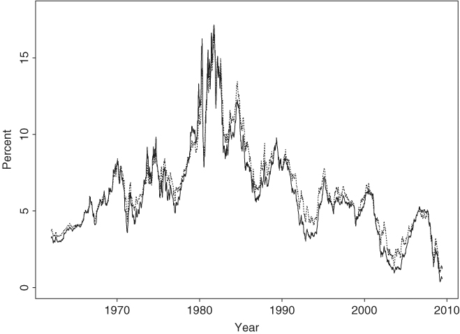
Figure 2.18 Scatterplots of U.S. weekly interest rates from January 5, 1962, to April 10, 2009: (a) 3-year rate vs. 1-year rate and (b) changes in 3-year rate vs. changes in 1-year rate.

Figure 2.19 Residual series of linear regression (2.44) for two U.S. weekly interest rates: (a) time plot and (b) sample ACF.

The unit-root behavior of both interest rates and the residuals of Eq. (2.44) leads to the consideration of the change series of interest rates. Let

and consider the linear regression c3t = βc1t + et. Figure 2.20 shows time plots of the two change series, whereas Figure 2.18(b) provides a scatterplot between them. The change series remain highly correlated with a fitted linear regression model given by

2.45

with R2 = 82.5%. The standard error of the coefficient is 0.0073. This model further confirms the strong linear dependence between interest rates. Figure 2.21 shows the time plot and sample ACF of the residuals of Eq. (2.45). Once again, the ACF shows some significant serial correlations in the residuals, but magnitudes of the correlations are much smaller. This weak serial dependence in the residuals can be modeled by using the simple time series models discussed in the previous sections, and we have a linear regression with time series errors.

Figure 2.20 Time plots of change series of U.S. weekly interest rates from January 12, 1962, to April 10, 2009: (a) changes in Treasury 1-year constant maturity rate and (b) changes in Treasury 3-year constant maturity rate.

Figure 2.21 Residual series of linear regression (2.45) for two change series of U.S. weekly interest rates: (a) time plot and (b) sample ACF.

The main objective of this section is to discuss a simple approach for building a linear regression model with time series errors. The approach is straightforward. We employ a simple time series model discussed in this chapter for the residual series and estimate the whole model jointly. For illustration, consider the simple linear regression in Eq. (2.45). Because residuals of the model are serially correlated, we shall identify a simple ARMA model for the residuals. From the sample ACF of the residuals shown in Figure 2.21, we specify an MA(1) model for the residuals and modify the linear regression model to

2.46

where {at} is assumed to be a white noise series. In other words, we simply use an MA(1) model, without the constant term, to capture the serial dependence in the error term of Eq. (2.45). The resulting model is a simple example of linear regression with time series errors. In practice, more elaborated time series models can be added to a linear regression equation to form a general regression model with time series errors.

Estimating a regression model with time series errors was not easy before the advent of modern computers. Special methods such as the Cochrane–Orcutt estimator have been proposed to handle the serial dependence in the residuals; see Greene (2003, p. 273). By now, the estimation is as easy as that of other time series models. If the time series model used is stationary and invertible, then one can estimate the model jointly via the maximum-likelihood method. This is the approach we take by using either the SCA or R package. R and S-Plus demonstrations are given later. For the U.S. weekly interest rate data, the fitted version of model (2.46) is

2.47

with R2 = 83.1%. The standard errors of the parameters are 0.0075 and 0.0196, respectively. The model no longer has a significant lag-1 residual ACF, even though some minor residual serial correlations remain at lags 4, 6, and 7. The incremental improvement of adding additional MA parameters at lags 4, 6, and 7 to the residual equation is small and the result is not reported here.

Comparing the models in Eqs. (2.44), (2.45), and (2.47), we make the following observations. First, the high R2 96.5% and coefficient 0.930 of model (2.44) are misleading because the residuals of the model show strong serial correlations. Second, for the change series, R2 and the coefficient of c1t of models (2.45) and (2.47) are close. In this particular instance, adding the MA(1) model to the change series only provides a marginal improvement. This is not surprising because the estimated MA coefficient is small numerically, even though it is statistically highly significant. Third, the analysis demonstrates that it is important to check residual serial dependence in linear regression analysis.

From Eq. (2.47), the model shows that the two weekly interest rate series are related as

The interest rates are concurrently and serially correlated.

R Demonstration

The following output has been edited.

Summary

We outline a general procedure for analyzing linear regression models with time series errors:

To check the serial correlations of residuals, we recommend that the Ljung–Box statistics be used instead of the Durbin–Watson (DW) statistic because the latter only considers the lag-1 serial correlation. There are cases in which serial dependence in residuals appears at higher order lags. This is particularly so when the time series involved exhibits some seasonal behavior.

In S-Plus, regression models with time series errors can be analyzed by the command OLS (ordinary least squares) if the residuals assume an AR model. Also, to identify a lagged variable, the command is tslag, for example, y = tslag(r,1). For the interest rate series, the relevant commands follow, where % denotes explanation of the command:

See the output in the next section for more information.