
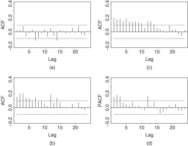
Let rt be the log return of an asset at time index t. The basic idea behind volatility study is that the series {rt} is either serially uncorrelated or with minor lower order serial correlations, but it is a dependent series. For illustration, consider the monthly log stock returns of Intel Corporation from January 1973 to December 2008 shown in Figure 3.1. Figure 3.2(a) shows the sample ACF of the log return series, which suggests no significant serial correlations except for a minor one at lag 7. Figure 3.2(c) shows the sample ACF of the absolute log returns (i.e., |rt|), whereas Figure 3.2(b) shows the sample ACF of the squared log returns ![]() . These two plots clearly suggest that the monthly log returns are not serially independent. Combining the three plots, it seems that the log returns are indeed serially uncorrelated but dependent. Volatility models attempt to capture such dependence in the return series.
. These two plots clearly suggest that the monthly log returns are not serially independent. Combining the three plots, it seems that the log returns are indeed serially uncorrelated but dependent. Volatility models attempt to capture such dependence in the return series.
Figure 3.1 Time plot of monthly log returns of Intel stock from January 1973 to December 2008.
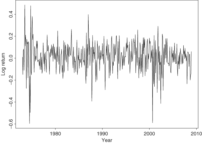
Figure 3.2 Sample ACF and PACF of various functions of monthly log stock returns of Intel Corporation from January 1973 to December 2008: (a) ACF of the log returns, (b) ACF of the squared log returns, (c) ACF of the absolute log returns, and (d) PACF of the squared log returns.
To put the volatility models in proper perspective, it is informative to consider the conditional mean and variance of rt given Ft−1; that is,
where Ft−1 denotes the information set available at time t − 1. Typically, Ft−1 consists of all linear functions of the past returns. As shown by the empirical examples of Chapter 2 and Figure 3.2, serial dependence of a stock return series rt is weak if it exists at all. Therefore, the equation for μt in (3.2) should be simple, and we assume that rt follows a simple time series model such as a stationary ARMA(p, q) model with some explanatory variables. In other words, we entertain the model
for rt, where k, p, and q are nonnegative integers, and xit are explanatory variables. Here yt is simply a notation representing the adjusted return series after removing the effect of explanatory variables.
Model (3.3) illustrates a possible financial application of the regression model with time series errors of Chapter 2. The order (p, q) of an ARMA model may depend on the frequency of the return series. For example, daily returns of a market index often show some minor serial correlations, but monthly returns of the index may not contain any significant serial correlation. The explanatory variables xt in Eq. (3.3) are flexible. For example, a dummy variable can be used for the Mondays to study the effect of the weekend on daily stock returns. In the capital asset pricing model (CAPM), the mean equation of rt can be written as rt = ϕ0 + βrm, t + at, where rm, t denotes the market return.
Combining Eqs. (3.2) and (3.3), we have
(3.4) ![]()
The conditional heteroscedastic models of this chapter are concerned with the evolution of ![]() . The manner under which
. The manner under which ![]() evolves over time distinguishes one volatility model from another.
evolves over time distinguishes one volatility model from another.
Conditional heteroscedastic models can be classified into two general categories. Those in the first category use an exact function to govern the evolution of ![]() , whereas those in the second category use a stochastic equation to describe
, whereas those in the second category use a stochastic equation to describe ![]() . The GARCH model belongs to the first category, whereas the stochastic volatility model is in the second category.
. The GARCH model belongs to the first category, whereas the stochastic volatility model is in the second category.
Throughout the book, at is referred to as the shock or innovation of an asset return at time t and σt is the positive square root of ![]() . The model for μt in Eq. (3.3) is referred to as the mean equation for rt and the model for
. The model for μt in Eq. (3.3) is referred to as the mean equation for rt and the model for ![]() is the volatility equation for rt. Therefore, modeling conditional heteroscedasticity amounts to augmenting a dynamic equation, which governs the time evolution of the conditional variance of the asset return, to a time series model.
is the volatility equation for rt. Therefore, modeling conditional heteroscedasticity amounts to augmenting a dynamic equation, which governs the time evolution of the conditional variance of the asset return, to a time series model.