
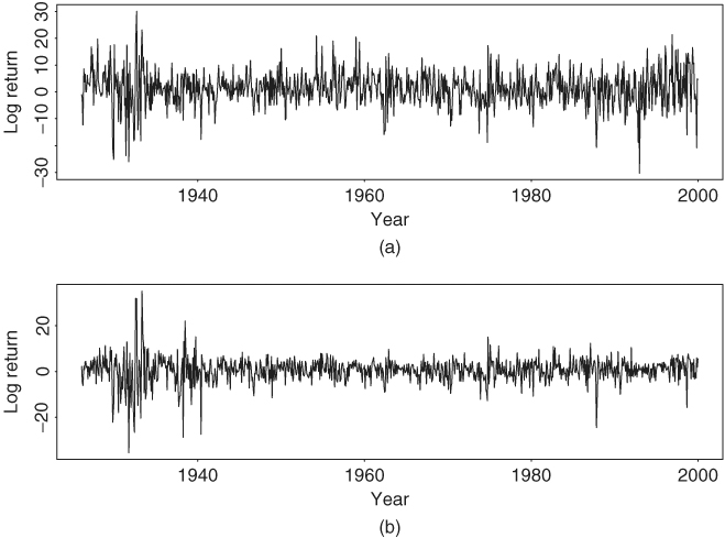
In this section, we apply the volatility models discussed in this chapter to investigate some problems of practical importance. The data used are the monthly log returns of IBM stock and the S&P 500 index from January 1926 to December 1999. There are 888 observations, and the returns are in percentages and include dividends. Figure 3.11 shows the time plots of the two return series. Note that the result of this section was obtained by the RATS program.
Figure 3.11 Time plots of monthly log returns for (a) IBM stock and (b) S&P 500 index. Sample period is from January 1926 to December 1999. Returns are in percentages and include dividends.
Example 3.4
The questions we address here are whether the daily volatility of a stock is lower in the summer and, if so, by how much. Affirmative answers to these two questions have practical implications in stock option pricing. We use the monthly log returns of IBM stock shown in Figure 3.11(a) as an illustrative example.
Denote the monthly log return series by rt. If Gaussian GARCH models are entertained, we obtain the GARCH(1,1) model:
for the series. The standard errors of the two parameters in the mean equation are 0.222 and 0.037, respectively, whereas those of the parameters in the volatility equation are 0.947, 0.021, and 0.037, respectively. Using the standardized residuals ãt = at/σt, we obtain Q(10) = 7.82(0.553) and Q(20) = 21.22(0.325), where the p value is in parentheses. Therefore, there are no serial correlations in the residuals of the mean equation. The Ljung–Box statistics of the ![]() series show Q(10) = 2.89(0.98) and Q(20) = 7.26(0.99), indicating that the standardized residuals have no conditional heteroscedasticity. The fitted model seems adequate. This model serves as a starting point for further study.
series show Q(10) = 2.89(0.98) and Q(20) = 7.26(0.99), indicating that the standardized residuals have no conditional heteroscedasticity. The fitted model seems adequate. This model serves as a starting point for further study.
To study the summer effect on stock volatility of an asset, we define an indicator variable
3.43 ![]()
and modify the volatility equation to
![]()
This equation uses two GARCH(1,1) models to describe the volatility of a stock return; one model for the summer months and the other for the remaining months. For the monthly log returns of IBM stock, estimation results show that the estimates of α10 and β10 are statistically nonsignificant at the 10% level. Therefore, we refine the equation and obtain the model
The standard errors of the parameters in the mean equation are 0.218 and 0.037, respectively, and those of the parameters in the volatility equation are 1.071, 0.022, 0.037, and 1.900, respectively. The Ljung–Box statistics for the standardized residuals ãt = at/σt show Q(10) = 7.66(0.569) and Q(20) = 21.64(0.302). Therefore, there are no serial correlations in the standardized residuals. The Ljung–Box statistics for ![]() give Q(10) = 3.38(0.97) and Q(20) = 6.82(0.99), indicating no conditional heteroscedasticity in the standardized residuals either. The refined model seems adequate.
give Q(10) = 3.38(0.97) and Q(20) = 6.82(0.99), indicating no conditional heteroscedasticity in the standardized residuals either. The refined model seems adequate.
Comparing the volatility models in Eqs. (3.42) and (3.44), we obtain the following conclusions. First, because the coefficient − 5.514 is significantly different from zero with a p value of 0.0067, the summer effect on stock volatility is statistically significant at the 1% level. Furthermore, the negative sign of the estimate confirms that the volatility of IBM monthly log stock returns is indeed lower during the summer. Second, rewrite the volatility model in Eq. (3.44) as
![]()
The negative constant term − 0.615 = 4.539 − 5.514 is counterintuitive. However, since the standard errors of 4.539 and 5.514 are relatively large, the estimated difference − 0.615 might not be significantly different from zero. To verify the assertion, we refit the model by imposing the constraint that the constant term of the volatility equation is zero for the summer months. This can easily be done by using the equation
![]()
The fitted model is
The standard errors of the parameters in the mean equation are 0.219 and 0.038, respectively, and those of the parameters in the volatility equation are 0.022, 0.034, and 1.094, respectively. The Ljung–Box statistics of the standardized residuals show Q(10) = 7.68 and Q(20) = 21.67, and those of the ![]() series give Q(10) = 3.17 and Q(20) = 6.85. These test statistics are close to what we had before and are not significant at the 5% level.
series give Q(10) = 3.17 and Q(20) = 6.85. These test statistics are close to what we had before and are not significant at the 5% level.
The volatility Eq. (3.45) can readily be used to assess the summer effect on the IBM stock volatility. For illustration, based on the model in Eq. (3.45) the medians of ![]() and
and ![]() are 29.4 and 75.1, respectively, for the IBM monthly log returns in 1999. Using these values, we have
are 29.4 and 75.1, respectively, for the IBM monthly log returns in 1999. Using these values, we have ![]() = 0.114 × 29.4 + 0.811 × 75.1 = 64.3 for the summer months and
= 0.114 × 29.4 + 0.811 × 75.1 = 64.3 for the summer months and ![]() = 68.8 for the other months. The ratio of the two volatilities is 64.3/68.8 ≈ 93%. Thus, there is a 7% reduction in the volatility of the monthly log return of IBM stock in the summer months.
= 68.8 for the other months. The ratio of the two volatilities is 64.3/68.8 ≈ 93%. Thus, there is a 7% reduction in the volatility of the monthly log return of IBM stock in the summer months.
Example 3.5
The S&P 500 index is widely used in the derivative markets. As such, modeling its volatility is a subject of intensive study. The question we ask in this example is whether the past returns of individual components of the index contribute to the modeling of the S&P 500 index volatility in the presence of its own returns. A thorough investigation on this topic is beyond the scope of this chapter, but we use the past returns of IBM stock as explanatory variables to address the question.
The data used are shown in Figure 3.11. Denote by rt the monthly log return series of the S&P 500 index. Using the rt series and Gaussian GARCH models, we obtain the following special GARCH(2,1) model:
The standard error of the constant term in the mean equation is 0.138, and those of the parameters in the volatility equation are 0.214, 0.021, and 0.017, respectively. Based on the standardized residuals ãt = at/σt, we have Q(10) = 11.51(0.32) and Q(20) = 23.71(0.26), where the number in parentheses denotes the p value. For the ![]() series, we have Q(10) = 9.42(0.49) and Q(20) = 13.01(0.88). Therefore, the model seems adequate at the 5% significance level.
series, we have Q(10) = 9.42(0.49) and Q(20) = 13.01(0.88). Therefore, the model seems adequate at the 5% significance level.
Next, we evaluate the contributions, if any, of using the past returns of IBM stock, which is a component of the S&P 500 index, in modeling the index volatility. As a simple illustration, we modify the volatility equation as
![]()
where xt is the monthly log return of IBM stock and 1.24 is the sample mean of xt. The fitted model for rt becomes
The standard error of the parameter in the mean equation is 0.139 and the standard errors of the parameters in the volatility equation are 0.271, 0.020, 0.018, and 0.002, respectively. For model checking, we have Q(10) = 11.39(0.33) and Q(20) = 23.63(0.26) for the standardized residuals ãt = at/σt and Q(10) = 9.35(0.50) and Q(20) = 13.51(0.85) for the ![]() series. Therefore, the model is adequate.
series. Therefore, the model is adequate.
Since the p value for testing γ = 0 is 0.0039, the contribution of the lag-1 IBM stock return to the S&P 500 index volatility is statistically significant at the 1% level. The negative sign is understandable because it implies that using the lag-1 past return of IBM stock reduces the volatility of the S&P 500 index return. Table 3.4 gives the fitted volatility of the S&P 500 index from July to December of 1999 using models (3.46) and (3.47). From the table, the past value of IBM log stock return indeed contributes to the modeling of the S&P 500 index volatility.
Table 3.4 Fitted Volatilities for Monthly Log Returns of S&P 500 Index from July to December 1999 Using Models with and without Past Log Return of IBM Stock
