
Most nonlinear models developed in the statistical literature focus on the conditional mean equation in Eq. (4.3); see Priestley (1988) and Tong (1990) for summaries of nonlinear models. Our goal here is to introduce some nonlinear models that are applicable to financial time series.
4.1.1 Bilinear Model
The linear model in Eq. (4.1) is simply the first-order Taylor series expansion of the f( · ) function in Eq. (4.2). As such, a natural extension to nonlinearity is to employ the second-order terms in the expansion to improve the approximation. This is the basic idea of bilinear models, which can be defined as
where p, q, m, and s are nonnegative integers. This model was introduced by Granger and Andersen (1978) and has been widely investigated. Subba Rao and Gabr (1984) discuss some properties and applications of the model, and Liu and Brockwell (1988) study general bilinear models. Properties of bilinear models such as stationarity conditions are often derived by (a) putting the model in a state-space form (see Chapter 11) and (b) using the state transition equation to express the state as a product of past innovations and random coefficient vectors. A special generalization of the bilinear model in Eq. (4.4) has conditional heteroscedasticity. For example, consider the model
4.5 ![]()
where {at} is a white noise series. The first two conditional moments of xt are
![]()
which are similar to that of the RCA or CHARMA model of Chapter 3.
Example 4.1
Consider the monthly simple returns of the CRSP equal-weighted index from January 1926 to December 2008 for 996 observations. Denote the series by Rt. The sample PACF of Rt shows significant partial autocorrelations at lags 1 and 3 so that an AR(3) model is used. The squared series of the AR(3) residuals suggests that the conditional heteroscedasticity might depend on lags 1, 3, and 8 of the residuals. Therefore, we employ the special bilinear model
![]()
for the series, where at = β0ϵt with ϵt being an iid series with mean zero and variance 1. Note that lag 8 is omitted for simplicity. Assuming that the conditional distribution of at is normal, we use the conditional maximum-likelihood method and obtain the fitted model
where the standard errors of the parameters are, in the order of appearance, 0.0023, 0.032, 0.027, 0.002, 0.147, and 0.136, respectively. All estimates are significantly different from zero at the 5% level. Define
![]()
where ![]() for t ≤ 3, as the standardized residual series of the model. The sample ACF of
for t ≤ 3, as the standardized residual series of the model. The sample ACF of ![]() shows no significant serial correlations, but the series is not independent because the squared series
shows no significant serial correlations, but the series is not independent because the squared series ![]() has significant serial correlations. The validity of model (4.6) deserves further investigation. For comparison, we also consider an AR(3)–ARCH(3) model for the series and obtain
has significant serial correlations. The validity of model (4.6) deserves further investigation. For comparison, we also consider an AR(3)–ARCH(3) model for the series and obtain
where all estimates but the coefficients of Rt−2 and Rt−3 are highly significant. The standardized residual series of the model shows no serial correlations, but the squared residuals show Q(10) = 19.78 with a p value of 0.031. Models (4.6) and (4.7) appear to be similar, but the latter seems to fit the data better. Further study shows that an AR(1)–GARCH(1,1) model fits the data well.
4.1.2 Threshold Autoregressive (TAR) Model
This model is motivated by several nonlinear characteristics commonly observed in practice such as asymmetry in declining and rising patterns of a process. It uses piecewise linear models to obtain a better approximation of the conditional mean equation. However, in contrast to the traditional piecewise linear model that allows for model changes to occur in the “time” space, the TAR model uses threshold space to improve linear approximation. Let us start with a simple 2-regime AR(1) model:
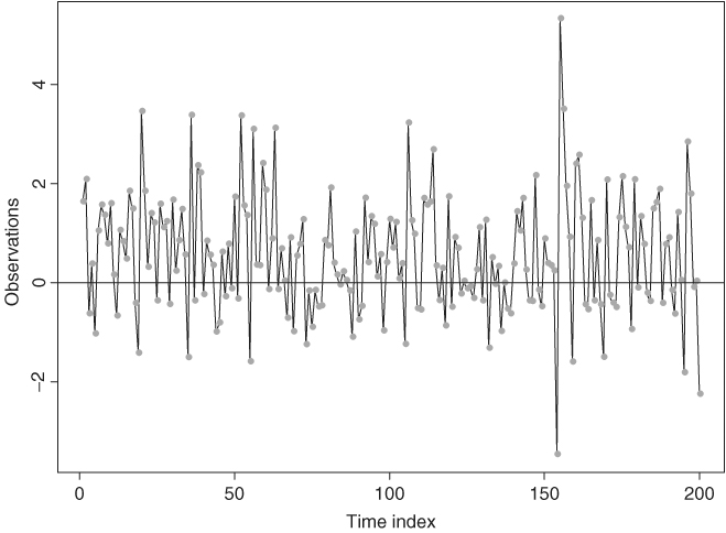
where the at are iid N(0, 1). Here the threshold variable is xt−1 so that the delay is 1, and the threshold is 0. Figure 4.1 shows the time plot of a simulated series of xt with 200 observations. A horizontal line of zero is added to the plot, which illustrates several characteristics of TAR models. First, despite the coefficient − 1.5 in the first regime, the process xt is geometrically ergodic and stationary. In fact, the necessary and sufficient condition for model (4.8) to be geometrically ergodic is ![]() ,
, ![]() , and
, and ![]() , where
, where ![]() is the AR coefficient of regime i; see Petruccelli and Woolford (1984) and Chen and Tsay (1991). Ergodicity is an important concept in time series analysis. For example, the statistical theory showing that the sample mean
is the AR coefficient of regime i; see Petruccelli and Woolford (1984) and Chen and Tsay (1991). Ergodicity is an important concept in time series analysis. For example, the statistical theory showing that the sample mean ![]() of xt converges to the mean of xt is referred to as the ergodic theorem, which can be regarded as the counterpart of the central limit theory for the iid case. Second, the series exhibits an asymmetric increasing and decreasing pattern. If xt−1 is negative, then xt tends to switch to a positive value due to the negative and explosive coefficient − 1.5. Yet when xt−1 is positive, it tends to take multiple time indexes for xt to reduce to a negative value. Consequently, the time plot of xt shows that regime 2 has more observations than regime 1, and the series contains large upward jumps when it becomes negative. The series is therefore not time reversible. Third, the model contains no constant terms, but E(xt) is not zero. The sample mean of the particular realization is 0.61 with a standard deviation of 0.07. In general, E(xt) is a weighted average of the conditional means of the two regimes, which are nonzero. The weight for each regime is simply the probability that xt is in that regime under its stationary distribution. It is also clear from the discussion that, for a TAR model to have zero mean, nonzero constant terms in some of the regimes are needed. This is very different from a stationary linear model for which a nonzero constant implies that the mean of xt is not zero.
of xt converges to the mean of xt is referred to as the ergodic theorem, which can be regarded as the counterpart of the central limit theory for the iid case. Second, the series exhibits an asymmetric increasing and decreasing pattern. If xt−1 is negative, then xt tends to switch to a positive value due to the negative and explosive coefficient − 1.5. Yet when xt−1 is positive, it tends to take multiple time indexes for xt to reduce to a negative value. Consequently, the time plot of xt shows that regime 2 has more observations than regime 1, and the series contains large upward jumps when it becomes negative. The series is therefore not time reversible. Third, the model contains no constant terms, but E(xt) is not zero. The sample mean of the particular realization is 0.61 with a standard deviation of 0.07. In general, E(xt) is a weighted average of the conditional means of the two regimes, which are nonzero. The weight for each regime is simply the probability that xt is in that regime under its stationary distribution. It is also clear from the discussion that, for a TAR model to have zero mean, nonzero constant terms in some of the regimes are needed. This is very different from a stationary linear model for which a nonzero constant implies that the mean of xt is not zero.
Figure 4.1 Time plot of simulated 2-regime TAR(1) series.
A time series xt is said to follow a k-regime self-exciting TAR (SETAR) model with threshold variable xt−d if it satisfies
where k and d are positive integers, j = 1, … , k, γi are real numbers such that − ∞ = γ0 < γ1 < ⋯ < γk−1 < γk = ∞, the superscript (j) is used to signify the regime, and ![]() are iid sequences with mean 0 and variance
are iid sequences with mean 0 and variance ![]() and are mutually independent for different j. The parameter d is referred to as the delay parameter and γj are the thresholds. Here it is understood that the AR models are different for different regimes; otherwise, the number of regimes can be reduced. Equation (4.9) says that a SETAR model is a piecewise linear AR model in the threshold space. It is similar in spirit to the usual piecewise linear models in regression analysis, where model changes occur in the order in which observations are taken. The SETAR model is nonlinear provided that k > 1.
and are mutually independent for different j. The parameter d is referred to as the delay parameter and γj are the thresholds. Here it is understood that the AR models are different for different regimes; otherwise, the number of regimes can be reduced. Equation (4.9) says that a SETAR model is a piecewise linear AR model in the threshold space. It is similar in spirit to the usual piecewise linear models in regression analysis, where model changes occur in the order in which observations are taken. The SETAR model is nonlinear provided that k > 1.
Properties of general SETAR models are hard to obtain, but some of them can be found in Tong (1990), Chan (1993), Chan and Tsay (1998), and the references therein. In recent years, there is increasing interest in TAR models and their applications; see, for instance, Hansen (1997), Tsay (1998), and Montgomery et al. (1998). Tsay (1989) proposed a testing and modeling procedure for univariate SETAR models. The model in Eq. (4.9) can be generalized by using a threshold variable zt that is measurable with respect to Ft−1 (i.e., a function of elements of Ft−1). The main requirements are that zt is stationary with a continuous distribution function over a compact subset of the real line and that zt−d is known at time t. Such a generalized model is referred to as an open-loop TAR model.
Example 4.2
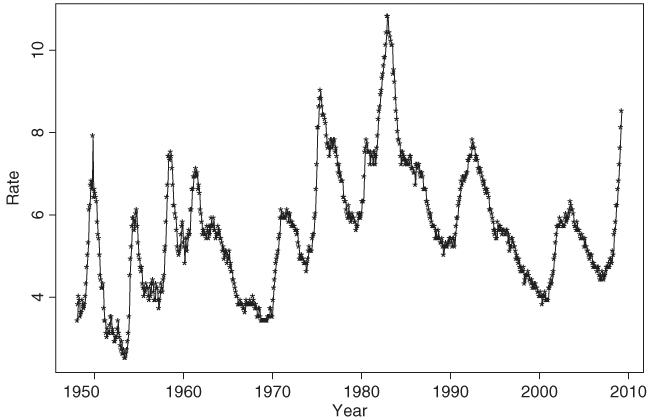
To demonstrate the application of TAR models, consider the U.S. monthly civilian unemployment rate, seasonally adjusted and measured in percentage, from January 1948 to March 2009 for 735 observations. The data are obtained from the Bureau of Labor Statistics, Department of Labor, and are shown in Figure 4.2. The plot shows two main characteristics of the data. First, there appears to be a slow but upward trend in the overall unemployment rate. Second, the unemployment rate tends to increase rapidly and decrease slowly. Thus, the series is not time reversible and may not be unit-root stationary, either.
Figure 4.2 Time plot of monthly U.S. civilian unemployment rate, seasonally adjusted, from January 1948 to March 2009.
Because the sample autocorrelation function decays slowly, we employ the first differenced series yt = (1 − B)ut in the analysis, where ut is the monthly unemployment rate. Using univariate ARIMA models, we obtain the model
where ![]() and all estimates but the AR(2) coefficient are statistically significant at the 5% level. The t ratio of the estimate of AR(2) coefficient is − 1.66. The residuals of model (4.10) give Q(12) = 12.3 and Q(24) = 25.5, respectively. The corresponding p values are 0.056 and 0.11, respectively, based on χ2 distributions with 6 and 18 degrees of freedom. Thus, the fitted model adequately describes the serial dependence of the data. Note that the seasonal AR and MA coefficients are highly significant with standard error 0.049 and 0.035, respectively, even though the data were seasonally adjusted. The adequacy of seasonal adjustment deserves further study. Using model (4.10), we obtain the 1-step-ahead forecast of 8.8 for the April 2009 unemployment rate, which is close to the actual data of 8.9.
and all estimates but the AR(2) coefficient are statistically significant at the 5% level. The t ratio of the estimate of AR(2) coefficient is − 1.66. The residuals of model (4.10) give Q(12) = 12.3 and Q(24) = 25.5, respectively. The corresponding p values are 0.056 and 0.11, respectively, based on χ2 distributions with 6 and 18 degrees of freedom. Thus, the fitted model adequately describes the serial dependence of the data. Note that the seasonal AR and MA coefficients are highly significant with standard error 0.049 and 0.035, respectively, even though the data were seasonally adjusted. The adequacy of seasonal adjustment deserves further study. Using model (4.10), we obtain the 1-step-ahead forecast of 8.8 for the April 2009 unemployment rate, which is close to the actual data of 8.9.
To model nonlinearity in the data, we employ TAR models and obtain the model
where the standard errors of ait are 0.180 and 0.217, respectively, the standard errors of the AR parameters in regime 1 are 0.046, 0.043, 0.042, and 0.037, whereas those of the AR parameters in regime 2 are 0.054, 0.057, and 0.075, respectively. The number of data points in regimes 1 and 2 are 460 and 262, respectively. The standardized residuals of model (4.11) only shows some minor serial correlation at lag 12. Based on the fitted TAR model, the dynamic dependence in the data appears to be stronger when the change in monthly unemployment rate is greater than 0.1%. This is understandable because a substantial increase in the unemployment rate is indicative of weakening in the U.S. economy, and policy makers might be more inclined to take action to help the economy, which in turn may affect the dynamics of the unemployment rate series. Consequently, model (4.11) is capable of describing the time-varying dynamics of the U.S. unemployment rate.
The MA representation of model (4.10) is
![]()
It is then not surprising to see that no yt−1 term appears in model (4.11).
As mentioned in Chapter 3, threshold models can be used in finance to handle the asymmetric responses in volatility between positive and negative returns. The models can also be used to study arbitrage tradings in index futures and cash prices; see Chapter 8 on multivariate time series analysis. Here we focus on volatility modeling and introduce an alternative approach to parameterization of TGARCH models. In some applications, this new general TGARCH model fares better than the GJR model of Chapter 3.
Example 4.3
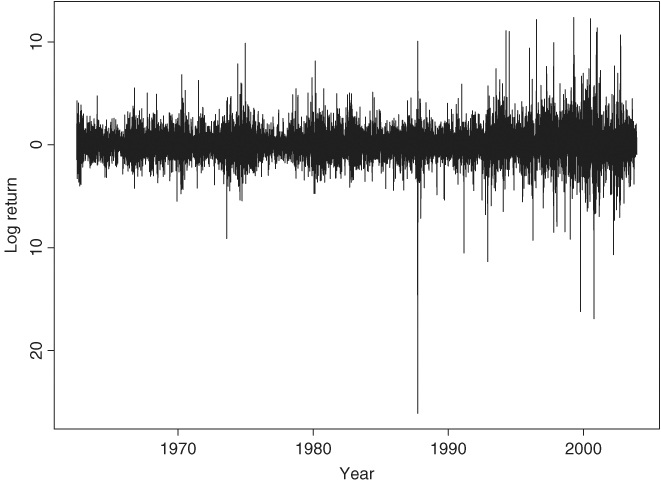
Consider the daily log returns, in percentage and including dividends, of IBM stock from July 3, 1962, to December 31, 2003, for 10,446 observations. Figure 4.3 shows the time plot of the series, which is one of the longer return series analyzed in the book. The volatility seems to be larger in the latter years of the data. Because general TGARCH models are used in the analysis, we use the SCA package to perform estimation in this example.
Figure 4.3 Time plot of daily log returns for IBM stock from July 3, 1962, to December 31, 2003.
If GARCH models of Chapter 3 are entertained, we obtain the following AR(2)–GARCH(1,1) model for the series:
where rt is the log return, {ϵt} is a Gaussian white noise sequence with mean zero and variance 1.0, the standard errors of the parameters in the mean equation are 0.015 and 0.010, and those of the volatility equation are 0.004, 0.003, and 0.003, respectively. All estimates are statistically significant at the 5% level. The Ljung–Box statistics of the standardized residuals give Q(10) = 5.19(0.82) and Q(20) = 24.38(0.18), where the number in parentheses denotes the p value obtained using ![]() distribution because of the estimated AR(2) coefficient. For the squared standardized residuals, we obtain Q(10) = 11.67(0.31) and Q(20) = 18.25(0.57). The model is adequate in modeling the serial dependence and conditional heteroscedasticity of the data. But the unconditional mean for rt of model (4.12) is 0.060, which is substantially larger than the sample mean 0.039, indicating that the model might be misspecified.
distribution because of the estimated AR(2) coefficient. For the squared standardized residuals, we obtain Q(10) = 11.67(0.31) and Q(20) = 18.25(0.57). The model is adequate in modeling the serial dependence and conditional heteroscedasticity of the data. But the unconditional mean for rt of model (4.12) is 0.060, which is substantially larger than the sample mean 0.039, indicating that the model might be misspecified.
Next, we employ the TGARCH model of Chapter 3 and obtain
where Pt−1 = 1 − Nt−1, Nt−1 is the indicator for negative at−1 such that Nt−1 = 1 if at−1 < 0 and = 0 otherwise, the standard errors of the parameters in the mean equation are 0.013 and 0.009, and those of the volatility equation are 0.007, 0.008, 0.010, and 0.010, respectively. All estimates except the constant term of the mean equation are significant. Let ãt be the standardized residuals of model (4.13). We have Q(10) = 2.47(0.98) and Q(20) = 25.90(0.13) for the {ãt} series and Q(10) = 97.07(0.00) and Q(20) = 170.3(0.00) for ![]() . The model fails to describe the conditional heteroscedasticity of the data.
. The model fails to describe the conditional heteroscedasticity of the data.
The idea of TAR models can be used to refine the prior TGARCH model by allowing for increased flexibility in modeling the asymmetric response in volatility. More specifically, we consider an AR(2)−TAR−GARCH(1,1) model for the series and obtain
where Nt−1 is defined in Eq. (4.13). All estimates in model (4.14) are significantly different from zero at the usual 1% level. Let ât be the standardized residuals of model (4.14). We obtain Q(10) = 6.09(0.73) and Q(20) = 25.29(0.15) for {ât} and Q(10) = 13.54(0.20) and Q(20) = 19.56(0.49) for ![]() . Thus, model (4.14) is adequate in modeling the serial correlation and conditional heteroscedasticity of the daily log returns of IBM stock considered. The unconditional mean return of model (4.14) is 0.033, which is much closer to the sample mean 0.039 than those implied by models (4.12) and (4.13). Comparing the two fitted TGARCH models, we see that the asymmetric behavior in daily IBM stock volatility is much stronger than what is allowed in a GJR model. Specifically, the coefficient of
. Thus, model (4.14) is adequate in modeling the serial correlation and conditional heteroscedasticity of the daily log returns of IBM stock considered. The unconditional mean return of model (4.14) is 0.033, which is much closer to the sample mean 0.039 than those implied by models (4.12) and (4.13). Comparing the two fitted TGARCH models, we see that the asymmetric behavior in daily IBM stock volatility is much stronger than what is allowed in a GJR model. Specifically, the coefficient of ![]() also depends on the sign of at−1. Note that model (4.14) can be further refined by imposing the constraint that the sum of the coefficients of
also depends on the sign of at−1. Note that model (4.14) can be further refined by imposing the constraint that the sum of the coefficients of ![]() and
and ![]() is one when at−1 < 0.
is one when at−1 < 0.
Remark
A RATS program to estimate the AR(2)−TAR−GARCH(1,1) model used is given in Appendix 4.6. The results might be slightly different from those of SCA given in the text.
4.1.3 Smooth Transition AR (STAR) Model
A criticism of the SETAR model is that its conditional mean equation is not continuous. The thresholds {γj} are the discontinuity points of the conditional mean function μt. In response to this criticism, smooth TAR models have been proposed; see Chan and Tong (1986) and Teräsvirta (1994) and the references therein. A time series xt follows a 2-regime STAR(p) model if it satisfies
where d is the delay parameter, Δ and s are parameters representing the location and scale of model transition, and F( · ) is a smooth transition function. In practice, F( · ) often assumes one of three forms—namely, logistic, exponential, or a cumulative distribution function. From Eq. (4.15) and with 0 ≤ F( · ) ≤ 1, the conditional mean of a STAR model is a weighted linear combination between the following two equations:

The weights are determined in a continuous manner by F[(xt−d − Δ)/s]. The prior two equations also determine properties of a STAR model. For instance, a prerequisite for the stationarity of a STAR model is that all zeros of both AR polynomials are outside the unit circle. An advantage of the STAR model over the TAR model is that the conditional mean function is differentiable. However, experience shows that the transition parameters Δ and s of a STAR model are hard to estimate. In particular, most empirical studies show that standard errors of the estimates of Δ and s are often quite large, resulting in t ratios of about 1.0; see Teräsvirta (1994). This uncertainty leads to various complications in interpreting an estimated STAR model.
Example 4.4
To illustrate the application of STAR models in financial time series analysis, we consider the monthly simple stock returns for Minnesota Mining and Manufacturing (3M) Company from February 1946 to December 2008. If ARCH models are entertained, we obtain the following ARCH(2) model:
4.16 ![]()
where standard errors of the estimates are 0.002, 0.0003, 0.047, and 0.050, respectively. As discussed before, such an ARCH model fails to show the asymmetric responses of stock volatility to positive and negative prior shocks. The STAR model provides a simple alternative that may overcome this difficulty. Applying STAR models to the monthly returns of 3M stock, we obtain the model
4.17 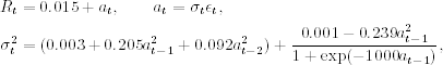
where the standard error of the constant term in the mean equation is 0.002 and the standard errors of the estimates in the volatility equation are 0.0002, 0.074, 0.043, 0.0004, and 0.080, respectively. The scale parameter 1000 of the logistic transition function is fixed a priori to simplify the estimation. This STAR model provides some support for asymmetric responses to positive and negative prior shocks. For a large negative at−1, the volatility model approaches the ARCH(2) model
![]()
Yet for a large positive at−1, the volatility process behaves like the ARCH(2) model
![]()
The negative coefficient of ![]() in the prior model is counterintuitive, but the magnitude is small. As a matter of fact, for a large positive shock at−1, the ARCH effects appear to be weak even though the parameter estimates remain statistically significant. The results shown are obtained using the command optim in R. A RATS program for estimating the STAR model is given in Appendix 4.6.
in the prior model is counterintuitive, but the magnitude is small. As a matter of fact, for a large positive shock at−1, the ARCH effects appear to be weak even though the parameter estimates remain statistically significant. The results shown are obtained using the command optim in R. A RATS program for estimating the STAR model is given in Appendix 4.6.
R Program for Estimating the STAR Model Used
> da=read.table(“m-3m4608.txt”,header=T)
> rtn=da[,2]
> source(“star.R”)
> par=c(.001,.002,.256,.141,.002,-.314)
> m2=optim(par,star,method=c(“BFGS”),hessian=T)
# function to calculate the likelihood of a STAR model.
star <- function(par){
f = 0
T1=length(rtn)
h=c(1,1)
at=c(0,0)
for (t in 3:T1){
resi = rtn[t]-par[1]
at=c(at,resi)
sig=par[2]+par[3]*at[t-1]ˆ2+par[4]*at[t-2]ˆ2
sig1=par[5]+par[6]*at[t-1]ˆ2
tt=sqrt(sig+sig1/(1+exp(-1000*at[t-1])))
h=c(h,tt)
x=resi/tt
f=f+log(tt)+0.5*x*x
}
f
}
4.1.4 Markov Switching Model
The idea of using probability switching in nonlinear time series analysis is discussed in Tong (1983). Using a similar idea, but emphasizing aperiodic transition between various states of an economy, Hamilton (1989) considers the Markov switching autoregressive (MSA) model. Here the transition is driven by a hidden two-state Markov chain. A time series xt follows an MSA model if it satisfies
where st assumes values in {1,2} and is a first-order Markov chain with transition probabilities
![]()
The innovational series {a1t} and {a2t} are sequences of iid random variables with mean zero and finite variance and are independent of each other. A small wi means that the model tends to stay longer in state i. In fact, 1/wi is the expected duration of the process to stay in state i. From the definition, an MSA model uses a hidden Markov chain to govern the transition from one conditional mean function to another. This is different from that of a SETAR model for which the transition is determined by a particular lagged variable. Consequently, a SETAR model uses a deterministic scheme to govern the model transition, whereas an MSA model uses a stochastic scheme. In practice, the stochastic nature of the states implies that one is never certain about which state xt belongs to in an MSA model. When the sample size is large, one can use some filtering techniques to draw inference on the state of xt. Yet as long as xt−d is observed, the regime of xt is known in a SETAR model. This difference has important practical implications in forecasting. For instance, forecasts of an MSA model are always a linear combination of forecasts produced by submodels of individual states. But those of a SETAR model only come from a single regime provided that xt−d is observed. Forecasts of a SETAR model also become a linear combination of those produced by models of individual regimes when the forecast horizon exceeds the delay d. It is much harder to estimate an MSA model than other models because the states are not directly observable. Hamilton (1990) uses the EM algorithm, which is a statistical method iterating between taking expectation and maximization. McCulloch and Tsay (1994) consider a Markov chain Monte Carlo (MCMC) method to estimate a general MSA model. We discuss MCMC methods in Chapter 12.
McCulloch and Tsay (1993) generalize the MSA model in Eq. (4.18) by letting the transition probabilities w1 and w2 be logistic, or probit, functions of some explanatory variables available at time t − 1. Chen, McCulloch, and Tsay (1997) use the idea of Markov switching as a tool to perform model comparison and selection between nonnested nonlinear time series models (e.g., comparing bilinear and SETAR models). Each competing model is represented by a state. This approach to select a model is a generalization of the odds ratio commonly used in Bayesian analysis. Finally, the MSA model can easily be generalized to the case of more than two states. The computational intensity involved increases rapidly, however. For more discussions of Markov switching models in econometrics, see Hamilton (1994, Chapter 22).
Example 4.5
Consider the growth rate, in percentages, of the U.S. quarterly real gross national product (GNP) from the second quarter of 1947 to the first quarter of 1991. The data are seasonally adjusted and shown in Figure 4.4, where a horizontal line of zero growth is also given. It is reassuring to see that a majority of the growth rates are positive. This series has been widely used in nonlinear analysis of economic time series. Tiao and Tsay (1994) and Potter (1995) use TAR models, whereas Hamilton (1989) and McCulloch and Tsay (1994) employ Markov switching models.
Figure 4.4 Time plot of growth rate of U.S. quarterly real GNP from 1947.II to 1991.I. Data are seasonally adjusted and in percentages.

Employing the MSA model in Eq. (4.18) with p = 4 and using a Markov chain Monte Carlo method, which is discussed in Chapter 12, McCulloch and Tsay (1994) obtain the estimates shown in Table 4.1. The results have several interesting findings. First, the mean growth rate of the marginal model for state 1 is 0.909/(1 − 0.265 − 0.029 + 0.126 + 0.11) = 0.965 and that of state 2 is − 0.42/(1 − 0.216 − 0.628 + 0.073 + 0.097) = − 1.288. Thus, state 1 corresponds to quarters with positive growth, or expansion periods, whereas state 2 consists of quarters with negative growth, or a contraction period. Second, the relatively large posterior standard deviations of the parameters in state 2 reflect that there are few observations in that state. This is expected as Figure 4.4 shows few quarters with negative growth. Third, the transition probabilities appear to be different for different states. The estimates indicate that it is more likely for the U.S. GNP to get out of a contraction period than to jump into one −0.286 versus 0.118. Fourth, treating 1/wi as the expected duration for the process to stay in state i, we see that the expected durations for a contraction period and an expansion period are approximately 3.69 and 11.31 quarters. Thus, on average, a contraction in the U.S. economy lasts about a year, whereas an expansion can last for 3 years. Finally, the estimated AR coefficients of xt−2 differ substantially between the two states, indicating that the dynamics of the U.S. economy are different between expansion and contraction periods.
Table 4.1 Estimation Results of Markov Switching Model with p = 4 for Growth Rate of U.S. Quarterly Real GNP, Seasonally Adjusteda

aThe estimates and their standard errors are posterior means and standard errors of a Gibbs sampling with 5000 iterations.
4.1.5 Nonparametric Methods
In some financial applications, we may not have sufficient knowledge to prespecify the nonlinear structure between two variables Y and X. In other applications, we may wish to take advantage of the advances in computing facilities and computational methods to explore the functional relationship between Y and X. These considerations lead to the use of nonparametric methods and techniques. Nonparametric methods, however, are not without cost. They are highly data dependent and can easily result in overfitting. Our goal here is to introduce some nonparametric methods for financial applications and some nonlinear models that make use of nonparametric methods and techniques. The nonparametric methods discussed include kernel regression, local least-squares estimation, and neural network.
The essence of nonparametric methods is smoothing. Consider two financial variables Y and X, which are related by
where m( · ) is an arbitrary, smooth, but unknown function and {at} is a white noise sequence. We wish to estimate the nonlinear function m( · ) from the data. For simplicity, consider the problem of estimating m( · ) at a particular date for which X = x. That is, we are interested in estimating m(x). Suppose that at X = x we have repeated independent observations y1, … , yT. Then the data become
![]()
Taking the average of the data, we have
![]()
By the law of large numbers, the average of the shocks converges to zero as T increases. Therefore, the average ![]() is a consistent estimate of m(x). That the average y provides a consistent estimate of m(x) or, alternatively, that the average of shocks converges to zero shows the power of smoothing.
is a consistent estimate of m(x). That the average y provides a consistent estimate of m(x) or, alternatively, that the average of shocks converges to zero shows the power of smoothing.
In financial time series, we do not have repeated observations available at X = x. What we observed are {(yt, xt)} for t = 1, … , T. But if the function m( · ) is sufficiently smooth, then the value of Yt for which Xt ≈ x continues to provide accurate approximation of m(x). The value of Yt for which Xt is far away from x provides less accurate approximation for m(x). As a compromise, one can use a weighted average of yt instead of the simple average to estimate m(x). The weight should be larger for those Yt with Xt close to x and smaller for those Yt with Xt far away from x. Mathematically, the estimate of m(x) for a given x can be written as
where the weights wt(x) are larger for those yt with xt close to x and smaller for those yt with xt far away from x. In Eq. (4.20), we assume that the weights sum to T. One can treat 1/T as part of the weights and make the weights sum to one.
From Eq. (4.20), the estimate ![]() is simply a local weighted average with weights determined by two factors. The first factor is the distance measure (i.e., the distance between xt and x). The second factor is the assignment of weight for a given distance. Different ways to determine the distance between xt and x and to assign the weight using the distance give rise to different nonparametric methods. In what follows, we discuss the commonly used kernel regression and local linear regression methods.
is simply a local weighted average with weights determined by two factors. The first factor is the distance measure (i.e., the distance between xt and x). The second factor is the assignment of weight for a given distance. Different ways to determine the distance between xt and x and to assign the weight using the distance give rise to different nonparametric methods. In what follows, we discuss the commonly used kernel regression and local linear regression methods.
Kernel Regression
Kernel regression is perhaps the most commonly used nonparametric method in smoothing. The weights here are determined by a kernel, which is typically a probability density function, is denoted by K(x), and satisfies
![]()
However, to increase the flexibility in distance measure, one often rescales the kernel using a variable h > 0, which is referred to as the bandwidth. The rescaled kernel becomes
The weight function can now be defined as
where the denominator is a normalization constant that makes the smoother adaptive to the local intensity of the X variable and ensures the weights sum to one. Plugging Eq. (4.22) into the smoothing formula (4.20), we have the well-known Nadaraya–Watson kernel estimator
4.23 ![]()
see Nadaraya (1964) and Watson (1964). In practice, many choices are available for the kernel K(x). However, theoretical and practical considerations lead to a few choices, including the Gaussian kernel
![]()
and the Epanechnikov kernel (Epanechnikov, 1969)
![]()
where I(A) is an indicator such that I(A) = 1 if A holds and I(A) = 0 otherwise. Figure 4.5 shows the Gaussian and Epanechnikov kernels for h = 1.
Figure 4.5 Standard normal kernel (solid line) and Epanechnikov kernel (dashed line) with bandwidth h = 1.

To understand the role played by the bandwidth h, we evaluate the Nadaraya–Watson estimator with the Epanechnikov kernel at the observed values {xt} and consider two extremes. First, if h → 0, then
![]()
indicating that small bandwidths reproduce the data. Second, if h → ∞, then
![]()
suggesting that large bandwidths lead to an oversmoothed curve—the sample mean. In general, the bandwidth function h acts as follows. If h is very small, then the weights focus on a few observations that are in the neighborhood around each xt. If h is very large, then the weights will spread over a larger neighborhood of xt. Consequently, the choice of h plays an important role in kernel regression. This is the well-known problem of bandwidth selection in kernel regression.
Bandwidth Selection
There are several approaches for bandwidth selection; see Härdle (1990) and Fan and Yao (2003). The first approach is the plug-in method, which is based on the asymptotic expansion of the mean integrated squared error (MISE) for kernel smoothers
![]()
where m( · ) is the true function. The quantity ![]() of the MISE is a pointwise measure of the mean squared error (MSE) of
of the MISE is a pointwise measure of the mean squared error (MSE) of ![]() evaluated at x. Under some regularity conditions, one can derive the optimal bandwidth that minimizes the MISE. The optimal bandwidth typically depends on several unknown quantities that must be estimated from the data with some preliminary smoothing. Several iterations are often needed to obtain a reasonable estimate of the optimal bandwidth. In practice, the choice of preliminary smoothing can become a problem. Fan and Yao (2003) give a normal reference bandwidth selector as
evaluated at x. Under some regularity conditions, one can derive the optimal bandwidth that minimizes the MISE. The optimal bandwidth typically depends on several unknown quantities that must be estimated from the data with some preliminary smoothing. Several iterations are often needed to obtain a reasonable estimate of the optimal bandwidth. In practice, the choice of preliminary smoothing can become a problem. Fan and Yao (2003) give a normal reference bandwidth selector as
![]()
where s is the sample standard error of the independent variable, which is assumed to be stationary.
The second approach to bandwidth selection is the leave-one-out cross validation. First, one observation (xj, yj) is left out. The remaining T − 1 data points are used to obtain the following smoother at xj:
![]()
which is an estimate of yj, where the weights wt(xj) sum to T − 1. Second, perform step 1 for j = 1, … , T and define the function
![]()
where W( · ) is a nonnegative weight function satisfying ![]() , that can be used to down-weight the boundary points if necessary. Decreasing the weights assigned to data points close to the boundary is needed because those points often have fewer neighboring observations. The function CV(h) is called the cross-validation function because it validates the ability of the smoother to predict
, that can be used to down-weight the boundary points if necessary. Decreasing the weights assigned to data points close to the boundary is needed because those points often have fewer neighboring observations. The function CV(h) is called the cross-validation function because it validates the ability of the smoother to predict ![]() . One chooses the bandwidth h that minimizes the CV(·) function.
. One chooses the bandwidth h that minimizes the CV(·) function.
Local Linear Regression Method
Assume that the second derivative of m( · ) in model (4.19) exists and is continuous at x, where x is a given point in the support of m( · ). Denote the data available by ![]() . The local linear regression method to nonparametric regression is to find a and b that minimize
. The local linear regression method to nonparametric regression is to find a and b that minimize
where Kh( · ) is a kernel function defined in Eq. (4.21) and h is a bandwidth. Denote the resulting value of a by â. The estimate of m(x) is then defined as â. In practice, x assumes an observed value of the independent variable. The estimate ![]() can be used as an estimate of the first derivative of m( · ) evaluated at x.
can be used as an estimate of the first derivative of m( · ) evaluated at x.
Under the least-squares theory, Eq. (4.24) is a weighted least-squares problem and one can derive a closed-form solution for a. Specifically, taking the partial derivatives of L(a, b) with respect to both a and b and equating the derivatives to zero, we have a system of two equations with two unknowns:
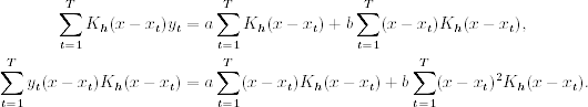
Define
![]()
The prior system of equations becomes
![]()
Consequently, we have
![]()
The numerator and denominator of the prior fraction can be further simplified as

In summary, we have
4.25 ![]()
where wt is defined as
![]()
In practice, to avoid possible zero in the denominator, we use the following ![]() to estimate m(x):
to estimate m(x):
Notice that a nice feature of Eq. (4.26) is that the weight wt satisfies
![]()
Also, if one assumes that m( · ) of Eq. (4.19) has the first derivative and finds the minimizer of
![]()
then the resulting estimator is the Nadaraya–Watson estimator mentioned earlier. In general, if one assumes that m(x) has a bounded kth derivative, then one can replace the linear polynomial in Eq. (4.24) by a (k − 1)-order polynomial. We refer to the estimator in Eq. (4.26) as the local linear regression smoother. Fan (1993) shows that, under some regularity conditions, the local linear regression estimator has some important sampling properties. The selection of bandwidth can be carried out via the same methods as before.
Time Series Application
In time series analysis, the explanatory variables are often the lagged values of the series. Consider the simple case of a single explanatory variable. Here model (4.19) becomes
![]()
and the kernel regression and local linear regression method discussed before are directly applicable. When multiple explanatory variables exist, some modifications are needed to implement the nonparametric methods. For the kernel regression, one can use a multivariate kernel such as a multivariate normal density function with a prespecified covariance matrix:
![]()
where p is the number of explanatory variables and Σ is a prespecified positive-definite matrix. Alternatively, one can use the product of univariate kernel functions as a multivariate kernel—for example,
![]()
This latter approach is simple, but it overlooks the relationship between the explanatory variables.
Example 4.6
To illustrate the application of nonparametric methods in finance, consider the weekly 3-month Treasury bill secondary market rate from 1970 to 1997 for 1461 observations. The data are obtained from the Federal Reserve Bank of St. Louis and are shown in Figure 4.6. This series has been used in the literature as an example of estimating stochastic diffusion equations using discretely observed data. See references in Chapter 6. Here we consider a simple model
![]()
where xt is the 3-month Treasury bill rate, yt = xt − xt−1, wt is a standard Brownian motion, and μ( · ) and σ( · ) are smooth functions of xt−1, and apply the local smoothing function lowess of R or S-Plus to obtain nonparametric estimates of μ( · ) and σ( · ); see Cleveland (1979). For simplicity, we use |yt| as a proxy of the volatility of xt.
Figure 4.6 Time plot of U.S. weekly 3-month Treasury bill rate in secondary market from 1970 to 1997.

For the simple model considered, μ(xt−1) is the conditional mean of yt given xt−1, that is, μ(xt−1) = E(yt|xt−1). Figure 4.7(a) shows the scatterplot of y(t) versus xt−1. The plot also contains the local smooth estimate of μ(xt−1) obtained by lowess of R or S-Plus. The estimate is essentially zero. However, to better understand the estimate, Figure 4.7(b) shows the estimate ![]() on a finer scale. It is interesting to see that
on a finer scale. It is interesting to see that ![]() is positive when xt−1 is small but becomes negative when xt−1 is large. This is in agreement with the common sense that when the interest rate is high, it is expected to come down, and when the rate is low, it is expected to increase. Figure 4.7(c) shows the scatterplot of |y(t)| versus xt−1 and the estimate of
is positive when xt−1 is small but becomes negative when xt−1 is large. This is in agreement with the common sense that when the interest rate is high, it is expected to come down, and when the rate is low, it is expected to increase. Figure 4.7(c) shows the scatterplot of |y(t)| versus xt−1 and the estimate of ![]() via lowess. The plot confirms that the higher the interest rate, the larger the volatility. Figure 4.7(d) shows the estimate
via lowess. The plot confirms that the higher the interest rate, the larger the volatility. Figure 4.7(d) shows the estimate ![]() on a finer scale. Clearly, the volatility is an increasing function of xt−1 and the slope seems to accelerate when xt−1 is approaching 10%. This example demonstrates that simple nonparametric methods can be helpful in understanding the dynamic structure of a financial time series.
on a finer scale. Clearly, the volatility is an increasing function of xt−1 and the slope seems to accelerate when xt−1 is approaching 10%. This example demonstrates that simple nonparametric methods can be helpful in understanding the dynamic structure of a financial time series.
Figure 4.7 Estimation of conditional mean and volatility of weekly 3-month Treasury bill rate via a local smoothing method: (a) yt vs. xt−1, where yt = xt − xt−1 and xt is interest rate; (b) estimate of μ(xt−1); (c) |yt| vs. xt−1; and (d) estimate of σ(xt−1).

R and S-Plus Commands Used in Example 4.6
> z1=read.table(‘w-3mtbs7097.txt’,header=T)
> x=z1[4,1:1460]/100
> y=(z1[4,2:1461]-z1[4,1:1460])/100
> par(mfcol=c(2,2))
> plot(x,y,pch=‘*’,xlab=‘x(t-1)’,ylab=‘y(t)’)
> lines(lowess(x,y))
> title(main=‘(a) y(t) vs x(t-1)’)
> fit=lowess(x,y)
> plot(fit$x,fit$y,xlab=‘x(t-1)’,ylab=‘mu’,type=‘l’,
+ ylim=c(-.002,.002))
> title(main=‘(b) Estimate of mu(.)’)
> plot(x,abs(y),pch=‘*’,xlab=‘x(t-1)’,ylab=‘abs(y)’)
> lines(lowess(x,abs(y)))
> title(main=‘(c) abs(y) vs x(t-1)’)
> fit2=lowess(x,abs(y))
> plot(fit2$x,fit2$y,type=‘l’,xlab=‘x(t-1)’,ylab=‘sigma’,
+ ylim=c(0,.01))
> title(main=‘(d) Estimate of sigma(.)’)
The following nonlinear models are derived with the help of nonparametric methods.
4.1.6 Functional Coefficient AR Model
Recent advances in nonparametric techniques enable researchers to relax parametric constraints in proposing nonlinear models. In some cases, nonparametric methods are used in a preliminary study to help select a parametric nonlinear model. This is the approach taken by Chen and Tsay (1993a) in proposing the functional coefficient autoregressive (FAR) model that can be written as
where Xt−1 = (xt−1, … , xt−k)′ is a vector of lagged values of xt. If necessary, Xt−1 may also include other explanatory variables available at time t − 1. The functions fi( · ) of Eq. (4.27) are assumed to be continuous, even twice differentiable, almost surely with respect to their arguments. Most of the nonlinear models discussed before are special cases of the FAR model. In application, one can use nonparametric methods such as kernel regression or local linear regression to estimate the functional coefficients fi( · ), especially when the dimension of Xt−1 is low (e.g., Xt−1 is a scalar). Recently, Cai, Fan, and Yao (2000) applied the local linear regression method to estimate fi( · ) and showed that substantial improvements in 1-step-ahead forecasts can be achieved by using FAR models.
4.1.7 Nonlinear Additive AR Model
A major difficulty in applying nonparametric methods to nonlinear time series analysis is the “curse of dimensionality.” Consider a general nonlinear AR(p) process xt = f(xt−1, … , xt−p) + at. A direct application of nonparametric methods to estimate f( · ) would require p-dimensional smoothing, which is hard to do when p is large, especially if the number of data points is not large. A simple, yet effective way to overcome this difficulty is to entertain an additive model that only requires lower dimensional smoothing. A time series xt follows a nonlinear additive AR (NAAR) model if
4.28 ![]()
where the fi( · ) are continuous functions almost surely. Because each function fi( · ) has a single argument, it can be estimated nonparametrically using one-dimensional smoothing techniques and hence avoids the curse of dimensionality. In application, an iterative estimation method that estimates fi( · ) nonparametrically conditioned on estimates of fj( · ) for all j ≠ i is used to estimate a NAAR model; see Chen and Tsay (1993b) for further details and examples of NAAR models.
The additivity assumption is rather restrictive and needs to be examined carefully in application. Chen, Liu, and Tsay (1995) consider test statistics for checking the additivity assumption.
4.1.8 Nonlinear State-Space Model
Making using of recent advances in MCMC methods (Gelfand and Smith, 1990), Carlin, Polson, and Stoffer (1992) propose a Monte Carlo approach for nonlinear state-space modeling. The model considered is
where St is the state vector, ft( · ) and gt( · ) are known functions depending on some unknown parameters, {ut} is a sequence of iid multivariate random vectors with zero mean and nonnegative definite covariance matrix Σu, {vt} is a sequence of iid random variables with mean zero and variance ![]() , and {ut} is independent of {vt}. Monte Carlo techniques are employed to handle the nonlinear evolution of the state transition equation because the whole conditional distribution function of St given St−1 is needed for a nonlinear system. Other numerical smoothing methods for nonlinear time series analysis have been considered by Kitagawa (1998) and the references therein. MCMC methods (or computing-intensive numerical methods) are powerful tools for nonlinear time series analysis. Their potential has not been fully explored. However, the assumption of knowing ft( · ) and gt( · ) in model (4.29) may hinder practical use of the proposed method. A possible solution to overcome this limitation is to use nonparametric methods such as the analyses considered in FAR and NAAR models to specify ft( · ) and gt( · ) before using nonlinear state-space models.
, and {ut} is independent of {vt}. Monte Carlo techniques are employed to handle the nonlinear evolution of the state transition equation because the whole conditional distribution function of St given St−1 is needed for a nonlinear system. Other numerical smoothing methods for nonlinear time series analysis have been considered by Kitagawa (1998) and the references therein. MCMC methods (or computing-intensive numerical methods) are powerful tools for nonlinear time series analysis. Their potential has not been fully explored. However, the assumption of knowing ft( · ) and gt( · ) in model (4.29) may hinder practical use of the proposed method. A possible solution to overcome this limitation is to use nonparametric methods such as the analyses considered in FAR and NAAR models to specify ft( · ) and gt( · ) before using nonlinear state-space models.
4.1.9 Neural Networks
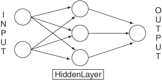
A popular topic in modern data analysis is neural networks, which can be classified as a semiparametric method. The literature on neural networks is enormous, and its application spreads over many scientific areas with varying degrees of success; see Section 2 of Ripley (1993) for a list of applications and Section 10 for remarks concerning its application in finance. Cheng and Titterington (1994) provide information on neural networks from a statistical viewpoint. In this subsection, we focus solely on the feed-forward neural networks in which inputs are connected to one or more neurons, or nodes, in the input layer, and these nodes are connected forward to further layers until they reach the output layer. Figure 4.8 shows an example of a simple feed-forward network for univariate time series analysis with one hidden layer. The input layer has two nodes, and the hidden layer has three. The input nodes are connected forward to each and every node in the hidden layer, and these hidden nodes are connected to the single node in the output layer. We call the network a 2–3–1 feed-forward network. More complicated neural networks, including those with feedback connections, have been proposed in the literature, but the feed-forward networks are most relevant to our study.
Figure 4.8 Feed-forward neural network with one hidden layer for univariate time series analysis.
Feed-Forward Neural Networks
A neural network processes information from one layer to the next by an “activation function.” Consider a feed-forward network with one hidden layer. The jth node in the hidden layer is defined as
4.30 
where xi is the value of the ith input node, fj( · ) is an activation function typically taken to be the logistic function
![]()
α0j is called the bias, the summation i → j means summing over all input nodes feeding to j, and wij are the weights. For illustration, the jth node of the hidden layer of the 2–3–1 feed-forward network in Figure 4.8 is
For the output layer, the node is defined as
4.32 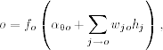
where the activation function fo( · ) is either linear or a Heaviside function. If fo( · ) is linear, then
![]()
where k is the number of nodes in the hidden layer. By a Heaviside function, we mean fo(z) = 1 if z > 0 and fo(z) = 0 otherwise. A neuron with a Heaviside function is called a threshold neuron, with 1 denoting that the neuron fires its message. For example, the output of the 2–3–1 network in Figure 4.8 is
![]()
if the activation function is linear; it is
![]()
if fo( · ) is a Heaviside function.
Combining the layers, the output of a feed-forward neural network can be written as

If one also allows for direct connections from the input layer to the output layer, then the network becomes
where the first summation is summing over the input nodes. When the activation function of the output layer is linear, the direct connections from the input nodes to the output node represent a linear function between the inputs and output. Consequently, in this particular case model (4.34) is a generalization of linear models. For the 2–3–1 network in Figure 4.8, if the output activation function is linear, then Eq. (4.33) becomes
![]()
where hj is given in Eq. (4.31). The network thus has 13 parameters. If Eq. (4.34) is used, then the network becomes
![]()
where again hj is given in Eq. (4.31). The number of parameters of the network increases to 15.
We refer to the function in Eq. (4.33) or (4.34) as a semiparametric function because its functional form is known, but the number of nodes and their biases and weights are unknown. The direct connections from the input layer to the output layer in Eq. (4.34) mean that the network can skip the hidden layer. We refer to such a network as a skip-layer feed-forward network.
Feed-forward networks are known as multilayer percetrons in the neural network literature. They can approximate any continuous function uniformly on compact sets by increasing the number of nodes in the hidden layer; see Hornik, Stinchcombe, and White (1989), Hornik (1993), and Chen and Chen (1995). This property of neural networks is the universal approximation property of the multilayer percetrons. In short, feed-forward neural networks with a hidden layer can be seen as a way to parameterize a general continuous nonlinear function.
Training and Forecasting
Application of neural networks involves two steps. The first step is to train the network (i.e., to build a network, including determining the number of nodes and estimating their biases and weights). The second step is inference, especially forecasting. The data are often divided into two nonoverlapping subsamples in the training stage. The first subsample is used to estimate the parameters of a given feed-forward neural network. The network so built is then used in the second subsample to perform forecasting and compute its forecasting accuracy. By comparing the forecasting performance, one selects the network that outperforms the others as the “best” network for making inference. This is the idea of cross validation widely used in statistical model selection. Other model selection methods are also available.
In a time series application, let {(rt, xt)|t= 1,… T} be the available data for network training, where xt denotes the vector of inputs and rt is the series of interest (e.g., log returns of an asset). For a given network, let ot be the output of the network with input ![]() ; see Eq. (4.34). Training a neural network amounts to choosing its biases and weights to minimize some fitting criterion—for example, the least squares
; see Eq. (4.34). Training a neural network amounts to choosing its biases and weights to minimize some fitting criterion—for example, the least squares
![]()
This is a nonlinear estimation problem that can be solved by several iterative methods. To ensure the smoothness of the fitted function, some additional constraints can be added to the prior minimization problem. In the neural network literature, the back propagation (BP) learning algorithm is a popular method for network training. The BP method, introduced by Bryson and Ho (1969), works backward starting with the output layer and uses a gradient rule to modify the biases and weights iteratively. Appendix 2A of Ripley (1993) provides a derivation of back propagation. Once a feed-forward neural network is built, it can be used to compute forecasts in the forecasting subsample.
Example 4.7
To illustrate applications of the neural network in finance, we consider the monthly log returns, in percentages and including dividends, for IBM stock from January 1926 to December 1999. We divide the data into two subsamples. The first subsample consisting of returns from January 1926 to December 1997 for 864 observations is used for modeling. Using model (4.34) with three inputs and two nodes in the hidden layer, we obtain a 3–2–1 network for the series. The three inputs are rt−1, rt−2, and rt−3 and the biases and weights are given next:
where rt-1 = (rt-1, rt-2, rt-3) and the two logistic functions are
The standard error of the residuals for the prior model is 6.56. For comparison, we also built an AR model for the data and obtained
The residual standard error is slightly greater than that of the feed-forward model in Eq. (4.35).
Forecast Comparison
The monthly returns of IBM stock in 1998 and 1999 form the second subsample and are used to evaluate the out-of-sample forecasting performance of neural networks. As a benchmark for comparison, we use the sample mean of rt in the first subsample as the 1-step-ahead forecast for all the monthly returns in the second subsample. This corresponds to assuming that the log monthly price of IBM stock follows a random walk with drift. The mean squared forecast error (MSFE) of this benchmark model is 91.85. For the AR(1) model in Eq. (4.36), the MSFE of 1-step-ahead forecasts is 91.70. Thus, the AR(1) model slightly outperforms the benchmark. For the 3–2–1 feed-forward network in Eq. (4.35), the MSFE is 91.74, which is essentially the same as that of the AR(1) model.
The estimation of feed-forward networks is done by using the nnet package of S-Plus with default starting weights; see Venables and Ripley (1999) for more information. Our limited experience shows that the estimation results vary. For the IBM stock returns used in Example 4.7, the out-of-sample MSE for a 3–2–1 network can be as low as 89.46 and as high as 93.65. If we change the number of nodes in the hidden layer, the range for the MSE becomes even wider. The S-Plus commands used in Example 4.7 are given in Appendix 4.7.
Example 4.8
Nice features of the feed-forward network include its flexibility and wide applicability. For illustration, we use the network with a Heaviside activation function for the output layer to forecast the direction of price movement for IBM stock considered in Example 4.7. Define a direction variable as
![]()
We use eight input nodes consisting of the first four lagged values of both rt and dt and four nodes in the hidden layer to build an 8–4–1 feed-forward network for dt in the first subsample. The resulting network is then used to compute the 1-step-ahead probability of an “upward movement” (i.e., a positive return) for the following month in the second subsample. Figure 4.9 shows a typical output of probability forecasts and the actual directions in the second subsample with the latter denoted by circles. A horizontal line of 0.5 is added to the plot. If we take a rigid approach by letting ![]() if the probability forecast is greater than or equal to 0.5 and
if the probability forecast is greater than or equal to 0.5 and ![]() otherwise, then the neural network has a successful rate of 0.58. The success rate of the network varies substantially from one estimation to another, and the network uses 49 parameters. To gain more insight, we did a simulation study of running the 8–4–1 feed-forward network 500 times and computed the number of errors in predicting the upward and downward movement using the same method as before. The mean and median of errors over the 500 runs are 11.28 and 11, respectively, whereas the maximum and minimum number of errors are 18 and 4. For comparison, we also did a simulation with 500 runs using a random walk with drift—that is,
otherwise, then the neural network has a successful rate of 0.58. The success rate of the network varies substantially from one estimation to another, and the network uses 49 parameters. To gain more insight, we did a simulation study of running the 8–4–1 feed-forward network 500 times and computed the number of errors in predicting the upward and downward movement using the same method as before. The mean and median of errors over the 500 runs are 11.28 and 11, respectively, whereas the maximum and minimum number of errors are 18 and 4. For comparison, we also did a simulation with 500 runs using a random walk with drift—that is,
![]()
where 1.19 is the average monthly log return for IBM stock from January 1926 to December 1997 and {ϵt} is a sequence of iid N(0, 1) random variables. The mean and median of the number of forecast errors become 10.53 and 11, whereas the maximum and minimum number of errors are 17 and 5, respectively. Figure 4.10 shows the histograms of the number of forecast errors for the two simulations. The results show that the 8–4–1 feed-forward neural network does not outperform the simple model that assumes a random walk with drift for the monthly log price of IBM stock.
Figure 4.9 One-step-ahead probability forecasts for positive monthly return for IBM stock using an 8–4–1 feed-forward neural network. Forecasting period is from January 1998 to December 1999.

Figure 4.10 Histograms of number of forecasting errors for directional movements of monthly log returns of IBM stock. Forecasting period is from January 1998 to December 1999.
