
In this section, we illustrate nonlinear time series models by analyzing the quarterly U.S. civilian unemployment rate, seasonally adjusted, from 1948 to 1993. This series was analyzed in detail by Montgomery et al. (1998). We repeat some of the analyses here using nonlinear models. Figure 4.11 shows the time plot of the data. Well-known characteristics of the series include that (a) it tends to move countercyclically with U.S. business cycles, and (b) the rate rises quickly but decays slowly. The latter characteristic suggests that the dynamic structure of the series is nonlinear.
Figure 4.11 Time plot of U.S. quarterly unemployment rate, seasonally adjusted, from 1948 to 1993.

Denote the series by xt and let Δxt = xt − xt−1 be the change in unemployment rate. The linear model
was built by Montgomery et al. (1998), where the standard errors of the three coefficients are 0.11, 0.06, and 0.07, respectively. This is a seasonal model even though the data were seasonally adjusted. It indicates that the seasonal adjustment procedure used did not successfully remove the seasonality. This model is used as a benchmark model for forecasting comparison.
To test for nonlinearity, we apply some of the nonlinearity tests of Section 4.2 with an AR(5) model for the differenced series Δxt. The results are given in Table 4.3. All of the tests reject the linearity assumption. In fact, the linearity assumption is rejected for all AR(p) models we applied, where p = 2, … , 10.
Table 4.3 Nonlinearity Test for Changes in the U.S. Quarterly Unemployment Rate: 1948.II–1993.IVa

aAn AR(5) model was used in the tests, where LST denotes the test of Luukkonen et al. (1988) and TAR(d) means threshold test with delay d.
Using a modeling procedure similar to that of Tsay (1989), Montgomery et al. (1998) build the following TAR model for the Δxt series:
The sample variances of a1t and a2t are 0.76 and 0.165, respectively, the standard errors of the three coefficients of regime 1 are 0.03, 0.10, and 0.12, respectively, and those of regime 2 are 0.09, 0.1, and 0.16. This model says that the change in the U.S. quarterly unemployment rate, Δxt, behaves like a piecewise linear model in the reference space of xt−2 − xt−3 with threshold 0.1. Intuitively, the model implies that the dynamics of unemployment act differently depending on the recent change in the unemployment rate. In the first regime, the unemployment rate has had either a decrease or a minor increase. Here the economy should be stable, and essentially the change in the rate follows a simple AR(1) model because the lag-2 coefficient is insignificant. In the second regime, there is a substantial jump in the unemployment rate (0.1 or larger). This typically corresponds to the contraction phase in the business cycle. It is also the period during which government interventions and industrial restructuring are likely to occur. Here Δxt follows an AR(2) model with a positive constant, indicating an upward trend in xt. The AR(2) polynomial contains two complex characteristic roots, which indicate possible cyclical behavior in Δxt. Consequently, the chance of having a turning point in xt increases, suggesting that the period of large increases in xt should be short. This implies that the contraction phases in the U.S. economy tend to be shorter than the expansion phases.
Applying a Markov chain Monte Carlo method, Montgomery et al. (1998) obtain the following Markov switching model for Δxt:
The conditional means of Δxt are − 0.10 for st = 1 and 0.31 for st = 2. Thus, the first state represents the expansionary periods in the economy, and the second state represents the contractions. The sample variances of ϵ1t and ϵ2t are 0.031 and 0.192, respectively. The standard errors of the three parameters in state st = 1 are 0.03, 0.14, and 0.11, and those of state st = 2 are 0.04, 0.13, and 0.14, respectively. The state transition probabilities are P(st = 2|st−1 = 1) = 0.084(0.060) and P(st = 1|st−1 = 2) = 0.126(0.053), where the number in parentheses is the corresponding standard error. This model implies that in the second state the unemployment rate xt has an upward trend with an AR(2) polynomial possessing complex characteristic roots. This feature of the model is similar to the second regime of the TAR model in Eq. (4.53). In the first state, the unemployment rate xt has a slightly decreasing trend with a much weaker autoregressive structure.
Forecasting Performance
A rolling procedure was used by Montgomery et al. (1998) to forecast the unemployment rate xt. The procedure works as follows:
1. Begin with forecast origin T = 83, corresponding to 1968.II, which was used in the literature to monitor the performance of various econometric models in forecasting unemployment rate. Estimate the linear, TAR, and MSA models using the data from 1948. I to the forecast origin (inclusive).
2. Perform 1-quarter to 5-quarter ahead forecasts and compute the forecast errors of each model. Forecasts of nonlinear models used are computed by using the parametric bootstrap method of Section 4.4.
3. Advance the forecast origin by 1 and repeat the estimation and forecasting processes until all data are employed.
4. Use MSE and mean forecast error to compare performance of the models.
Table 4.4 shows the relative MSE of forecasts and mean forecast errors for the linear model in Eq. (4.52), the TAR model in Eq. (4.53), and the MSA model in Eq. (4.54), using the linear model as a benchmark. The comparisons are based on overall performance as well as the status of the U.S. economy at the forecast origin. From the table, we make the following observations:
1. For the overall comparison, the TAR model and the linear model are very close in MSE, but the TAR model has smaller biases. Yet the MSA model has the highest MSE and smallest biases.
2. For forecast origins in economic contractions, the TAR model shows improvements over the linear model both in MSE and bias. The MSA model also shows some improvement over the linear model, but the improvement is not as large as that of the TAR model.
3. For forecast origins in economic expansions, the linear model outperforms both nonlinear models.
Table 4.4 Out-of-Sample Forecast Comparison among Linear, TAR, and MSA Models for the U.S. Quarterly Unemployment Ratea
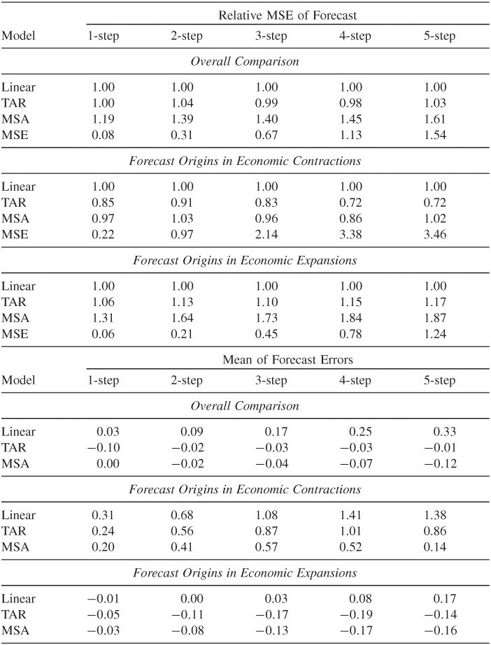
aThe starting forecast origin is 1968.II, where the row marked by MSE shows the MSE of the benchmark linear model.
The results suggest that the contributions of nonlinear models over linear ones in forecasting the U.S. quarterly unemployment rate are mainly in the periods when the U.S. economy is in contraction. This is not surprising because, as mentioned before, it is during the economic contractions that government interventions and industrial restructuring are most likely to occur. These external events could introduce nonlinearity in the U.S. unemployment rate. Intuitively, such improvements are important because it is during the contractions that people pay more attention to economic forecasts.