
5.3 Empirical Characteristics of Transactions Data
Let ti be the calendar time, measured in seconds from midnight, at which the ith transaction of an asset takes place. Associated with the transaction are several variables such as the transaction price, the transaction volume, the prevailing bid and ask quotes, and so on. The collection of ti and the associated measurements are referred to as the transactions data. These data have several important characteristics that do not exist when the observations are aggregated over time. Some of the characteristics are given next.
1. Unequally Spaced Time Intervals Transactions such as stock tradings on an exchange do not occur at equally spaced time intervals. As such, the observed transaction prices of an asset do not form an equally spaced time series. The time duration between trades becomes important and might contain useful information about market microstructure (e.g., trading intensity).
2. Discrete-Valued Prices The price change of an asset from one transaction to the next only occurred in multiples of tick size before January 29, 2001. On the NYSE, the tick size was one-eighth of a dollar before June 24, 1997 and was one-sixteenth of a dollar before January 29, 2001. Therefore, the price was a discrete-valued variable in transactions data. Although all equity markets in the United States now use the decimal system, the price change in consecutive trades tends to occur in multiples of one cent and can be treated approximately as a discrete-valued variable. In some markets, price change may also be subject to limit constraints set by regulators.
3. Existence of a Daily Periodic or Diurnal Pattern Under the normal trading conditions, transaction activity can exhibit a periodic pattern. For instance, on the NYSE, transactions are “heavier” at the beginning and closing of the trading hours and “thinner” during lunch hour, resulting in a U-shaped transaction intensity. Consequently, time durations between transactions also exhibit a daily cyclical pattern.
4. Multiple Transactions within a Single Second It is possible that multiple transactions, even with different prices, occur at the same time. This is partly due to the fact that time is measured in seconds, which may be too long a time scale in periods of heavy trading.
To demonstrate these characteristics, we consider first the IBM transactions data from November 1, 1990, to January 31, 1991. These data are from the Trades, Orders Reports, and Quotes (TORQ) data set; see Hasbrouck (1992). There are 63 trading days and 60,328 transactions. To simplify the discussion, we ignore the price changes between trading days and focus on the transactions that occurred in the normal trading hours from 9:30 am to 4:00 pm Eastern time. It is well known that overnight stock returns differ substantially from intraday returns; see Stoll and Whaley (1990) and the references therein. Table 5.1 gives the frequencies in percentages of price change measured in the tick size of ![]() . From the table, we make the following observations:
. From the table, we make the following observations:
1. About two-thirds of the intraday transactions were without price change.
2. The price changed in one tick approximately 29% of the intraday transactions.
3. Only 2.6% of the transactions were associated with two-tick price changes.
4. Only about 1.3% of the transactions resulted in price changes of three ticks or more.
5. The distribution of positive and negative price changes was approximately symmetric.
Table 5.1 Frequencies of Price Change in Multiples of Tick Size for IBM Stock from November 1, 1990, to January 31, 1991

Consider next the number of transactions in a 5-minute time interval. Denote the series by xt. That is, x1 is the number of IBM transactions from 9:30 am to 9:35 am on November 1, 1990, Eastern time; x2 is the number of transactions from 9:35 am to 9:40 am; and so on. The time gaps between trading days are ignored. Figure 5.1(a) shows the time plot of xt, and Figure 5.1(b) shows the sample ACF of xt for lags 1–260. Of particular interest is the cyclical pattern of the ACF with a periodicity of 78, which is the number of 5-minute intervals in a trading day. The number of transactions thus exhibits a daily pattern. To further illustrate the daily trading pattern, Figure 5.2 shows the average number of transactions within 5-minute time intervals over the 63 days. There are 78 such averages. The plot exhibits a “smiling” or U shape, indicating heavier trading at the opening and closing of the market and thinner trading during the lunch hours.
Figure 5.1 IBM intraday transactions data from 11/01/90 to 1/31/91: (a) number of transactions in 5-minute time intervals and (b) sample ACF of series in part (a).

Figure 5.2 Time plot of average number of transactions in 5-minute time intervals. There are 78 observations, averaging over 63 trading days from 11/01/90 to 1/31/91 for IBM stock.

Since we focus on transactions that occurred during normal trading hours of a trading day, there are 59,838 time intervals in the data. These intervals are called the intraday durations between trades. For IBM stock, there were 6531 zero time intervals. That is, during the normal trading hours of the 63 trading days from November 1, 1990, to January 31, 1991, multiple transactions in a second occurred 6531 times, which is about 10.91%. Among these multiple transactions, 1002 of them had different prices, which is about 1.67% of the total number of intraday transactions. Therefore, multiple transactions (i.e., zero durations) may become an issue in statistical modeling of the time durations between trades.
Table 5.2 provides a two-way classification of price movements. Here price movements are classified into “up,” “unchanged,” and “down.” We denote them by + , 0, and −, respectively. The table shows the price movements between two consecutive trades [i.e., from the (i − 1)th to the ith transaction] in the sample. From the table, trade-by-trade data show that:
1. Consecutive price increases or decreases are relatively rare, which are about 441/59837 = 0.74% and 410/59837 = 0.69%, respectively.
2. There is a slight edge to move from up to unchanged rather than to down; see row 1 of the table.
3. There is a high tendency for the price to remain unchanged.
4. The probabilities of moving from down to up or unchanged are about the same; see row 3.
Table 5.2 Two-Way Classification of Price Movements in Consecutive Intraday Trades for IBM Stocka

a The price movements are classified into “up,” “unchanged,” and “down.” The data span is from November 1, 1990, to January 31, 1991.
The first observation mentioned before is a clear demonstration of bid–ask bounce, showing price reversals in intraday transactions data. To confirm this phenomenon, we consider a directional series Di for price movements, where Di assumes the value + 1, 0, and − 1 for up, unchanged, and down price movement, respectively, for the ith transaction. The ACF of {Di} has a single spike at lag 1 with value − 0.389, which is highly significant for a sample size of 59,837 and confirms the price reversal in consecutive trades.
As a second illustration, we consider the transactions data of IBM stock in December 1999 obtained from the TAQ database. The normal trading hours are from 9:30 am to 4:00 pm Eastern time, except for December 31 when the market closed at 1:00 pm. Comparing with the 1990–1991 data, two important changes have occurred. First, the number of intraday tradings has increased sixfold. There were 134,120 intraday tradings in December 1999 alone. The increased trading intensity also increased the chance of multiple transactions within a second. The percentage of trades with zero time duration doubled to 22.98%. At the extreme, there were 42 transactions within a given second that happened twice on December 3, 1999. Second, the tick size of price movement was ![]() instead of
instead of ![]() . The change in tick size should reduce the bid–ask spread. Figure 5.3 shows the daily number of transactions in the new sample. Figure 5.4(a) shows the time plot of time durations between trades, measured in seconds, and Figure 5.4(b) is the time plot of price changes in consecutive intraday trades, measured in multiples of the tick size of
. The change in tick size should reduce the bid–ask spread. Figure 5.3 shows the daily number of transactions in the new sample. Figure 5.4(a) shows the time plot of time durations between trades, measured in seconds, and Figure 5.4(b) is the time plot of price changes in consecutive intraday trades, measured in multiples of the tick size of ![]() . As expected, Figures 5.3 and 5.4(a) show clearly the inverse relationship between the daily number of transactions and the time interval between trades. Figure 5.4(b) shows two unusual price movements for IBM stock on December 3, 1999. They were a drop of 63 ticks followed by an immediate jump of 64 ticks and a drop of 68 ticks followed immediately by a jump of 68 ticks. Unusual price movements like these occurred infrequently in intraday transactions.
. As expected, Figures 5.3 and 5.4(a) show clearly the inverse relationship between the daily number of transactions and the time interval between trades. Figure 5.4(b) shows two unusual price movements for IBM stock on December 3, 1999. They were a drop of 63 ticks followed by an immediate jump of 64 ticks and a drop of 68 ticks followed immediately by a jump of 68 ticks. Unusual price movements like these occurred infrequently in intraday transactions.
Figure 5.3 IBM transactions data for December 1999. Box plot shows the number of transactions in each trading day with after-hours portion denoting number of trades with time stamp after 4:00 PM.
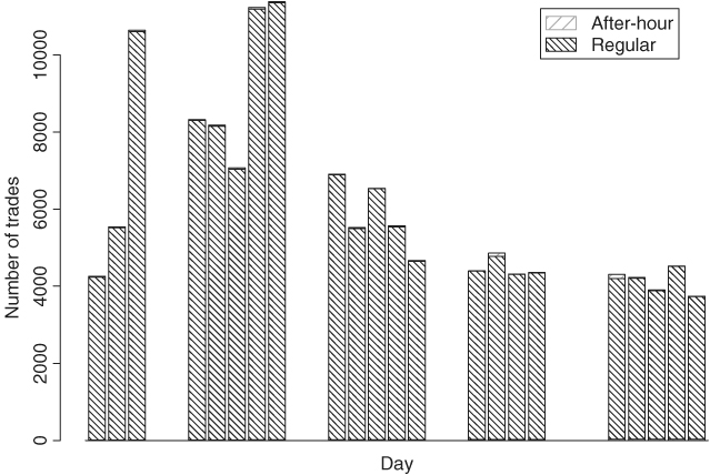
Figure 5.4 IBM transactions data for December 1999. (a) Time plot of time durations between trades and (b) time plot of price changes in consecutive trades measured in multiples of tick size of $1/16. Only data during normal trading hours are included.

Focusing on trades recorded within regular trading hours, we have 61,149 trades out of 133,475 with no price change. This is about 45.8% and substantially lower than that between November 1990 and January 1991. It seems that reducing the tick size increased the chance of a price change. Table 5.3 gives the percentages of trades associated with a price change. The price movements remain approximately symmetric with respect to zero. Large price movements in intraday tradings are still relatively rare.
Table 5.3 Percentages of Intraday Transactions Associated with a Price Change for IBM Stock Traded in December 1999a

aThe percentage of transactions without price change is 45.8% and the total number of transactions recorded within regular trading hours is 133,475. The size is measured in multiples of tick size $ 1/16.
Finally, we consider the transactions data of Boeing stock on December 1, 2008. There are 43,894 transactions within the regular trading hours. Figure 5.5(a) shows the transaction prices versus the calendar time measured in seconds from the midnight, and Figure 5.5(b) shows the time plot of price changes. In this particular instance, the price shows a downward trend within the day, but the price changes continue to exhibit patterns similar to those before using the decimal system. Figure 5.6 shows the histogram of the price changes for the Boeing stock. The histogram shows some distinct characteristics. First, the price changes appear to be symmetric with respective to zero. Second, the price changes indeed concentrate on multiples of one cent. Out of the 43,894 transactions, 58.5% have no price change; see the big spike of the histogram. Details of the summary of price changes for the Boeing stock are given in Table 5.4. The remaining 4.59% of the price changes not shown in Table 5.4 are not in multiples of one cent.
Figure 5.5 Transactions data of Boeing stock on December 1, 2008. (a) Price series over calendar time measured in seconds from midnight and (b) time plot of price changes in consecutive trades measured in cents. Only data during normal trading hours are included.
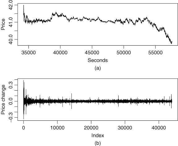
Figure 5.6 Histogram of price changes for Boeing stock on December 1, 2008.
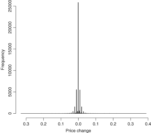
Table 5.4 Frequencies of Price Change for Boeing Stock on December 1, 2008

Remark
The recordkeeping of high-frequency data is often not as good as that of observations taken at lower frequencies. Data cleaning becomes a necessity in high-frequency data analysis. For transactions data, missing observations may happen in many ways, and the accuracy of the exact transaction time might be questionable for some trades. For example, recorded trading times may be beyond 4:00 pm Eastern time even before the opening of after-hours tradings. How to handle these observations deserves a careful study. A proper method of data cleaning requires a deep understanding of the way in which the market operates. As such, it is important to specify clearly and precisely the methods used in data cleaning. These methods must be taken into consideration in making inference.
Again, let ti be the calendar time, measured in seconds from midnight, when the ith transaction took place. Let ![]() be the transaction price. The price change from the (i − 1)th to the ith trade is yi
be the transaction price. The price change from the (i − 1)th to the ith trade is yi ![]() and the time duration is Δti = ti − ti−1. Here it is understood that the subscript i in Δti and yi denotes the time sequence of transactions, not the calendar time. In what follows, we consider models for yi and Δti both individually and jointly.
and the time duration is Δti = ti − ti−1. Here it is understood that the subscript i in Δti and yi denotes the time sequence of transactions, not the calendar time. In what follows, we consider models for yi and Δti both individually and jointly.