
Duration models are concerned with time intervals between trades. Longer durations indicate lack of trading activities, which in turn signify a period of no new information. The dynamic behavior of durations thus contains useful information about intraday market activities. Using concepts similar to the ARCH models for volatility, Engle and Russell (1998) propose an autoregressive conditional duration (ACD) model to describe the evolution of time durations for (heavily traded) stocks. Zhang et al. (2001) extend the ACD model to account for nonlinearity and structural breaks in the data. In this section, we introduce some simple duration models. As mentioned before, intraday transactions exhibit some diurnal pattern. Therefore, we focus on the adjusted time duration
where f(ti) is a deterministic function consisting of the cyclical component of Δti. Obviously, f(ti) depends on the underlying asset and the systematic behavior of the market. In practice, there are many ways to estimate f(ti), but no single method dominates the others in terms of statistical properties. A common approach is to use smoothing spline. Here we use simple quadratic functions and indicator variables to take care of the deterministic component of daily trading activities.
For the IBM data employed in the illustration of ADS models, we assume
where
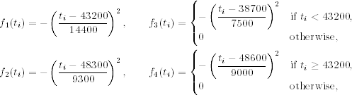
and f5(ti) and f6(ti) are indicator variables for the first and second 5 minutes of market opening [i.e., f5( · ) = 1 if and only if ti is between 9:30 am and 9:35 am Eastern time], and f7(ti) is the indicator for the last 30 minutes of daily trading [i.e., f7(ti) = 1 if and only if the trade occurred between 3:30 pm and 4:00 pm Eastern time]. Figure 5.7 shows the plot of fi( · ) for i = 1, … , 4, where the time scale on the x axis is in minutes. Note that f3(43200) = f4(43200), where 43,200 corresponds to 12:00 noon.
Figure 5.7 Quadratic functions used to remove deterministic component of IBM intraday trading durations: (a)–(d) are functions f1( · ) to f4( · ) of Eq. (5.32), respectively.
The coefficients βj of Eq. (5.32) are obtained by the least-squares method of the linear regression
![]()
The fitted model is
![]()
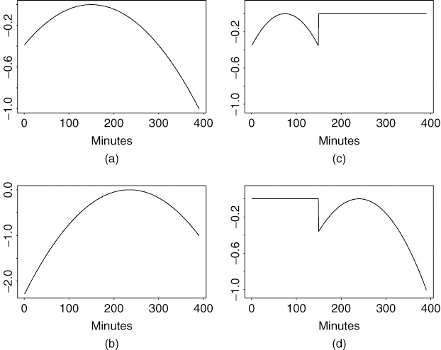
Figure 5.8 shows the time plot of average durations in 5-minute time intervals over the 63 trading days before and after adjusting for the deterministic component. Figure 5.8(a) shows the average durations of Δti and, as expected, exhibits a diurnal pattern. Figure 5.8(b) shows the average durations of ![]() (i.e., after the adjustment), and the diurnal pattern is largely removed.
(i.e., after the adjustment), and the diurnal pattern is largely removed.
Figure 5.8 IBM transactions data from 11/01/90 to 1/31/91: (a) average durations in 5-minute time intervals and (b) average durations in 5-minute time intervals after adjusting for deterministic component.
5.5.1 The ACD Model
The autoregressive conditional duration (ACD) model uses the idea of GARCH models to study the dynamic structure of the adjusted duration ![]() of Eq. (5.31). For ease in notation, we define
of Eq. (5.31). For ease in notation, we define ![]() .
.
Let ψi = E(xi|Fi−1) be the conditional expectation of the adjusted duration between the (i − 1)th and ith trades, where Fi−1 is the information set available at the (i − 1)th trade. In other words, ψi is the expected adjusted duration given Fi−1. The basic ACD model is defined as
5.33 ![]()
where {ϵi} is a sequence of independent and identically distributed nonnegative random variables such that E(ϵi) = 1. In Engle and Russell (1998), ϵi follows a standard exponential or a standardized Weibull distribution, and ψi assumes the form
5.34 ![]()
Such a model is referred to as an ACD(r, s) model. When the distribution of ϵi is exponential, the resulting model is called an EACD(r, s) model. Similarly, if ϵi follows a Weibull distribution, the model is a WACD(r, s) model. If necessary, readers are referred to Appendix A for a quick review of exponential and Weibull distributions.
Similar to GARCH models, the process ηi = xi − ψi is a martingale difference sequence [i.e., E(ηi|Fi−1) = 0], and the ACD(r, s) model can be written as
which is in the form of an ARMA process with non-Gaussian innovations. It is understood here that γj = 0 for j > r and ωj = 0 for j > s. Such a representation can be used to obtain the basic conditions for weak stationarity of the ACD model. For instance, taking expectation on both sides of Eq. (5.35) and assuming weak stationarity, we have
![]()
Therefore, we assume ω > 0 and 1 > ∑j(γj + ωj) because the expected duration is positive. As another application of Eq. (5.35), we study properties of the EACD(1,1) model.
EACD(1,1) Model
An EACD(1,1) model can be written as
where ϵi follows the standard exponential distribution. Using the moments of a standard exponential distribution in Appendix A, we have E(ϵi) = 1, Var(ϵi) = 1, and ![]() . Assuming that xi is weakly stationary (i.e., the first two moments of xi are time invariant), we derive the variance of xi. First, taking the expectation of Eq. (5.36), we have
. Assuming that xi is weakly stationary (i.e., the first two moments of xi are time invariant), we derive the variance of xi. First, taking the expectation of Eq. (5.36), we have
Under weak stationarity, E(ψi) = E(ψi−1) so that Eq. (5.37) gives
Next, because ![]() = 2, we have
= 2, we have ![]() .
.
Taking the square of ψi in Eq. (5.36) and the expectation and using weak stationarity of ψi and xi, we have, after some algebra, that
5.39 ![]()
Finally, using Var(xi) = ![]() and
and ![]() , we have
, we have
![]()
where μx is defined in Eq. (5.38). This result shows that, to have time-invariant unconditional variance, the EACD(1,1) model in Eq. (5.36) must satisfy ![]() . The variance of a WACD(1,1) model can be obtained by using the same techniques and the first two moments of a standardized Weibull distribution.
. The variance of a WACD(1,1) model can be obtained by using the same techniques and the first two moments of a standardized Weibull distribution.
ACD Models with a Generalized Gamma Distribution
In the statistical literature, intensity function is often expressed in terms of hazard function. As shown in Appendix B, the hazard function of an EACD model is constant over time and that of a WACD model is a monotonous function. These hazard functions are rather restrictive in application as the intensity function of stock transactions might not be constant or monotone over time. To increase the flexibility of the associated hazard function, Zhang et al. (2001) employ a (standardized) generalized gamma distribution for ϵi. See Appendix A for some basic properties of a generalized gamma distribution. The resulting hazard function may assume various patterns, including U shape or inverted U shape. We refer to an ACD model with innovations that follow a generalized gamma distribution as a GACD(r, s) model.
5.5.2 Simulation
To illustrate ACD processes, we generated 500 observations from the ACD(1,1) model:
using two different innovational distributions for ϵi. In case 1, ϵi is assumed to follow a standardized Weibull distribution with parameter α = 1.5. In case 2, ϵi follows a (standardized) generalized gamma distribution with parameters κ = 1.5 and α = 0.5.
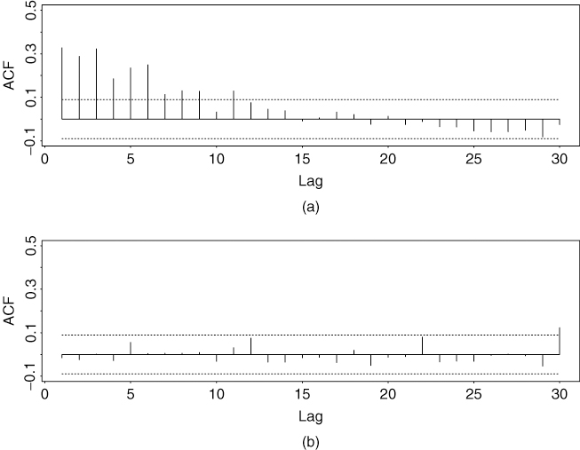
Figure 5.9(a) shows the time plot of the WACD(1,1) series, whereas Figure 5.10(a) is the GACD(1,1) series. Figure 5.11 plots the histograms of both simulated series. The difference between the two models is evident. Finally, the sample ACFs of the two simulated series are shown in Figures 5.12(a) and 5.13(b), respectively. The serial dependence of the data is clearly seen.
Figure 5.9 Simulated WACD(1,1) series in Eq. (5.40): (a) original series and (b) standardized series after estimation. There are 500 observations.
Figure 5.10 Simulated GACD(1,1) series in Eq. (5.40): (a) original series and (b) standardized series after estimation. There are 500 observations.
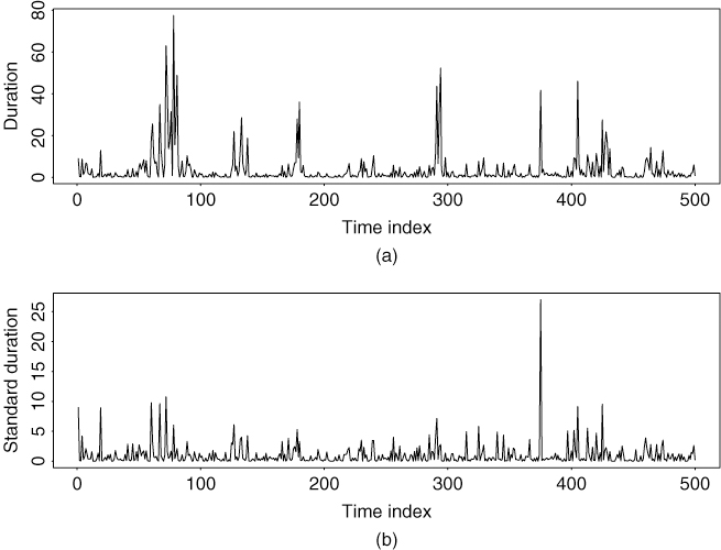
Figure 5.11 Histograms of simulated duration processes with 500 observations: (a) WACD(1,1) model and (b) GACD(1,1) model.
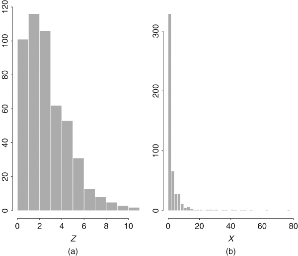
Figure 5.12 Sample autocorrelation function of simulated WACD(1,1) series with 500 observations: (a) original series and (b) standardized residual series.

Figure 5.13 Sample autocorrelation function of simulated GACD(1,1) series with 500 observations: (a) original series and (b) standardized residual series.
5.5.3 Estimation
For an ACD(r, s) model, let io = max(r, s) and xt = (x1, … , xt)′. The likelihood function of the durations x1, … , xT is
![]()
where θ denotes the vector of model parameters, and T is the sample size. The marginal probability density function ![]() of the previous equation is rather complicated for a general ACD model. Because its impact on the likelihood function is diminishing as the sample size T increases, this marginal density is often ignored, resulting in use of the conditional-likelihood method. For a WACD model, we use the probability density function (pdf) of Eq. (5.56) and obtain the conditional log-likelihood function
of the previous equation is rather complicated for a general ACD model. Because its impact on the likelihood function is diminishing as the sample size T increases, this marginal density is often ignored, resulting in use of the conditional-likelihood method. For a WACD model, we use the probability density function (pdf) of Eq. (5.56) and obtain the conditional log-likelihood function

where ![]() , θ = (ω, γ1,…,γr, ω,1,…,ωs, α,)′, and
, θ = (ω, γ1,…,γr, ω,1,…,ωs, α,)′, and ![]() . When α = 1, the (conditional) log-likelihood function reduces to that of an EACD(r, s) model.
. When α = 1, the (conditional) log-likelihood function reduces to that of an EACD(r, s) model.
For a GACD(r, s) model, the conditional log-likelihood function is
where λ = Γ(κ)/Γ(κ + 1/α) and the parameter vector θ now also includes κ. As expected, when κ = 1, λ = 1/Γ(1 + 1/α) and the log-likelihood function in Eq. (5.42) reduces to that of a WACD(r, s) model in Eq. (5.41). This log-likelihood function can be rewritten in many ways to simplify the estimation.
Under some regularity conditions, the conditional maximum-likelihood estimates are asymptotically normal; see Engle and Russell (1998) and the references therein. In practice, simulation can be used to obtain finite-sample reference distributions for the problem of interest once a duration model is specified.
Example 5.3
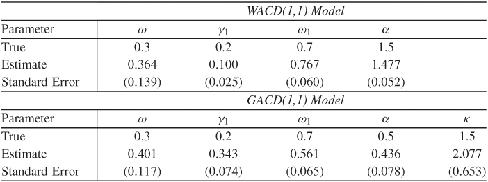
(Simulated ACD(1,1) series, continued). Consider the simulated WACD(1,1) and GACD(1,1) series of Eq. (5.40). We apply the conditional-likelihood method and obtain the results in Table 5.7. The estimates appear to be reasonable. Let ![]() be the 1-step-ahead prediction of ψi and
be the 1-step-ahead prediction of ψi and ![]() be the standardized series, which can be regarded as standardized residuals of the series. If the model is adequately specified,
be the standardized series, which can be regarded as standardized residuals of the series. If the model is adequately specified, ![]() should behave as a sequence of independent and identically distributed random variables. Figures 5.9(b) and 5.10(b) show the time plot of
should behave as a sequence of independent and identically distributed random variables. Figures 5.9(b) and 5.10(b) show the time plot of ![]() for both models. The sample ACF of
for both models. The sample ACF of ![]() for both fitted models are shown in Figures 5.12(b) and 5.13(b), respectively. It is evident that no significant serial correlations are found in the
for both fitted models are shown in Figures 5.12(b) and 5.13(b), respectively. It is evident that no significant serial correlations are found in the ![]() series.
series.
Table 5.7 Estimation Results for Simulated ACD(1,1) Series with 500 Observations: For WACD(1,1) Series and GACD(1,1) Series
Example 5.4
As an illustration of duration models, we consider the transaction durations of IBM stock on five consecutive trading days from November 1 to November 7, 1990. Focusing on positive transaction durations, we have 3534 observations. In addition, the data have been adjusted by removing the deterministic component in Eq. (5.32). That is, we employ 3534 positive adjusted durations as defined in Eq. (5.31).
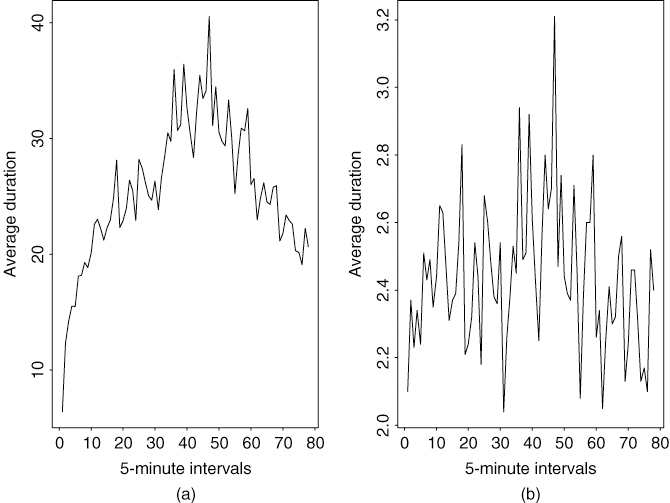
Figure 5.14(a) shows the time plot of the adjusted (positive) durations for the first five trading days of November 1990, and Figure 5.15(a) gives the sample ACF of the series. There exist some serial correlations in the adjusted durations. We fit a WACD(1,1) model to the data and obtain the model
where {ϵi} is a sequence of independent and identically distributed random variates that follow the standardized Weibull distribution with parameter ![]() = 0.879(0.012), where 0.012 is the estimated standard error. Standard errors of the estimates in Eq. (5.43) are 0.039, 0.010, and 0.018, respectively. All t ratios of the estimates are greater than 4.2, indicating that the estimates are significant at the 1% level. Figure 5.14(b) shows the time plot of
= 0.879(0.012), where 0.012 is the estimated standard error. Standard errors of the estimates in Eq. (5.43) are 0.039, 0.010, and 0.018, respectively. All t ratios of the estimates are greater than 4.2, indicating that the estimates are significant at the 1% level. Figure 5.14(b) shows the time plot of ![]() , and Figure 5.15(b) provides the sample ACF of
, and Figure 5.15(b) provides the sample ACF of ![]() . The Ljung–Box statistics show Q(10) = 4.96 and Q(20) = 10.75 for the
. The Ljung–Box statistics show Q(10) = 4.96 and Q(20) = 10.75 for the ![]() series. Clearly, the standardized innovations have no significant serial correlations. In fact, the sample autocorrelations of the squared series
series. Clearly, the standardized innovations have no significant serial correlations. In fact, the sample autocorrelations of the squared series ![]() are also small with Q(10) = 6.20 and Q(20) = 11.16, further confirming lack of serial dependence in the normalized innovations. In addition, the mean and standard deviation of a standardized Weibull distribution with α = 0.879 are 1.00 and 1.14, respectively. These numbers are close to the sample mean and standard deviation of
are also small with Q(10) = 6.20 and Q(20) = 11.16, further confirming lack of serial dependence in the normalized innovations. In addition, the mean and standard deviation of a standardized Weibull distribution with α = 0.879 are 1.00 and 1.14, respectively. These numbers are close to the sample mean and standard deviation of ![]() , which are 1.01 and 1.22, respectively. The fitted model seems adequate.
, which are 1.01 and 1.22, respectively. The fitted model seems adequate.
Figure 5.14 Time plots of durations for IBM stock traded in first five trading days of November 1990: (a) adjusted series and (b) normalized innovations of an WACD(1,1) model. There are 3534 nonzero durations.
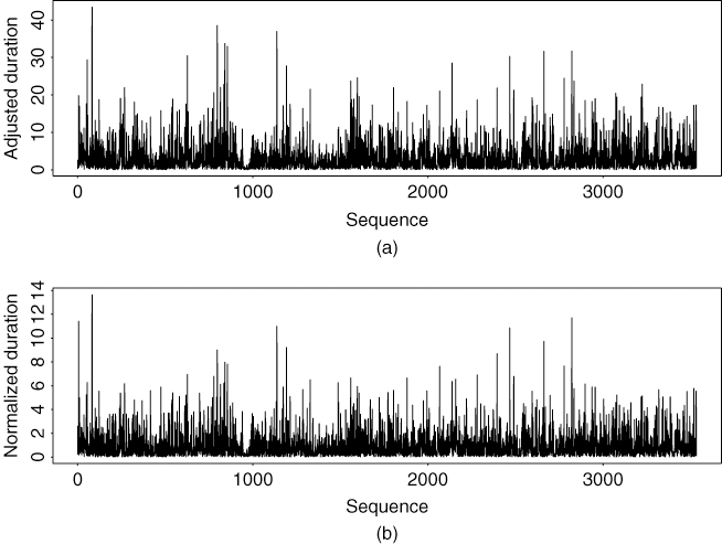
Figure 5.15 Sample autocorrelation function of adjusted durations for IBM stock traded in first five trading days of November 1990: (a) adjusted series and (b) normalized innovations for WACD(1,1) model.

In model (5.43), the estimated coefficients show ![]() 0.949, indicating certain persistence in the adjusted durations. The expected adjusted duration is 0.169/(1 − 0.064 − 0.885) = 3.31 seconds, which is close to the sample mean 3.29 of the adjusted durations. The estimated α of the standardized Weibull distribution is 0.879, which is less than but close to 1. Thus, the conditional hazard function is monotonously decreasing at a slow rate.
0.949, indicating certain persistence in the adjusted durations. The expected adjusted duration is 0.169/(1 − 0.064 − 0.885) = 3.31 seconds, which is close to the sample mean 3.29 of the adjusted durations. The estimated α of the standardized Weibull distribution is 0.879, which is less than but close to 1. Thus, the conditional hazard function is monotonously decreasing at a slow rate.
If a generalized gamma distribution function is used for the innovations, then the fitted GACD(1,1) model is
where {ϵi} follows a standardized, generalized gamma distribution in Eq. (5.57) with parameters κ = 4.248(1.046) and α = 0.395(0.053), where the number in parentheses denotes estimated standard error. Standard errors of the three parameters in Eq. (5.44) are 0.041, 0.010, and 0.019, respectively. All of the estimates are statistically significant at the 1% level. Again, the normalized innovational process ![]() and its squared series have no significant serial correlation, where
and its squared series have no significant serial correlation, where ![]() based on model (5.44). Specifically, for the
based on model (5.44). Specifically, for the ![]() process, we have Q(10) = 4.95 and Q(20) = 10.28. For the
process, we have Q(10) = 4.95 and Q(20) = 10.28. For the ![]() series, we have Q(10) = 6.36 and Q(20) = 10.89.
series, we have Q(10) = 6.36 and Q(20) = 10.89.
The expected duration of model (5.44) is 3.52, which is slightly greater than that of the WACD(1,1) model in Eq. (5.43). Similarly, the persistence parameter ![]() of model (5.44) is also slightly higher at 0.96.
of model (5.44) is also slightly higher at 0.96.
Remark
Estimation of EACD models can be carried out by using programs for ARCH models with some minor modification; see Engle and Russell (1998). In this book, we use either the RATS program or some Fortran programs developed by the author to estimate the duration models. Limited experience indicates that it is harder to estimate a GACD model than an EACD or a WACD model. RATS programs used to estimate WACD and GACD models are given in Appendix C.