
6.2 Some Continuous-Time Stochastic Processes
In mathematical statistics, a continuous-time continuous stochastic process is defined on a probability space (Ω, F, P), where Ω is a nonempty space, F is a σ field consisting of subsets of Ω, and P is a probability measure; see Chapter 1 of Billingsley (1986). The process can be written as {x(η, t)}, where t denotes time and is continuous in [0, ∞). For a given t, x(η, t) is a real-valued continuous random variable (i.e., a mapping from Ω to the real line), and η is an element of Ω. For the price of an asset at time t, the range of x(η, t) is the set of nonnegative real numbers. For a given η, {x(η, t)} is a time series with values depending on the time t. For simplicity, we write a continuous-time stochastic process as {xt} with the understanding that, for a given t, xt is a random variable. In the literature, some authors use x(t) instead of xt to emphasize that t is continuous. However, we use the same notation xt, but call it a continuous-time stochastic process.
6.2.1 Wiener Process
In a discrete-time econometric model, we assume that the shocks form a white noise process, which is not predictable. What is the counterpart of shocks in a continuous-time model? The answer is the increments of a Wiener process, which is also known as a standard Brownian motion. There are many ways to define a Wiener process {wt}. We use a simple approach that focuses on the small change Δwt = wt+Δt − wt associated with a small increment Δt in time. A continuous-time stochastic process {wt} is a Wiener process if it satisfies
1. ![]() , where ϵ is a standard normal random variable; and
, where ϵ is a standard normal random variable; and
2. Δwt is independent of wj for all j ≤ t.
The second condition is a Markov property saying that conditional on the present value wt, any past information of the process, wj with j < t, is irrelevant to the future wt+ℓ with ℓ > 0. From this property, it is easily seen that for any two nonoverlapping time intervals Δ1 and Δ2, the increments ![]() and
and ![]() are independent. In finance, this Markov property is related to a weak form of efficient market.
are independent. In finance, this Markov property is related to a weak form of efficient market.
From the first condition, Δwt is normally distributed with mean zero and variance Δt. That is, Δwt ∼ N(0, Δt), where ∼ denotes probability distribution. Consider next the process wt. We assume that the process starts at t = 0 with initial value w0, which is fixed and often set to zero. Then wt − w0 can be treated as a sum of many small increments. More specifically, define T = t/Δt, where Δt is a small positive increment. Then
![]()
where Δwi = wiΔt − w(i−1)Δt. Because the ϵi are independent, we have
![]()
Thus, the increment in wt from time 0 to time t is normally distributed with mean zero and variance t. To put it formally, for a Wiener process wt, we have that wt − w0 ∼ N(0, t). This says that the variance of a Wiener process increases linearly with the length of time interval.
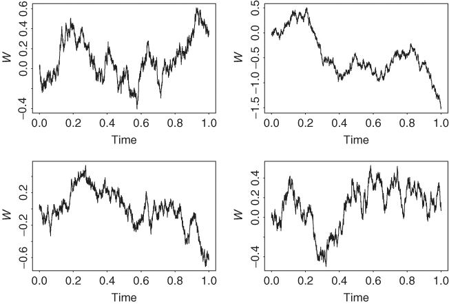
Figure 6.1 shows four simulated Wiener processes on the unit time interval [0, 1]. They are obtained by using a simple version of Donsker's theorem in the statistical literature with n = 3000; see Donsker (1951) or Billingsley (1968). The four plots start with w0 = 0 but drift apart as time increases, illustrating that the variance of a Wiener process increases with time. A simple time transformation from [0, 1) to [0, ∞) can be used to obtain simulated Wiener processes for t ∈ [0, ∞).
Figure 6.1 Four simulated Wiener processes.
Donsker's Theorem
Assume that ![]() is a sequence of independent standard normal random variates. For any t ∈ [0, 1], let [nt] be the integer part of nt. Define
is a sequence of independent standard normal random variates. For any t ∈ [0, 1], let [nt] be the integer part of nt. Define ![]() . Then wn, t converges in distribution to a Wiener process wt on [0, 1] as n goes to infinity.
. Then wn, t converges in distribution to a Wiener process wt on [0, 1] as n goes to infinity.
R or S-Plus Commands for Generating a Wiener Process
n = 3000
epsi = rnorm(n,0,1)
w=cumsum(epsi)/sqrt(n)
plot(w,type=‘l’)
Remark
A formal definition of a Brownian motion wt on a probability space (Ω, F, P) is that it is a real-valued, continuous stochastic process for t ≥ 0 with independent and stationary increments. In other words, wt satisfies the following:
1. Continuity: The map from t to wt is continuous almost surely with respect to the probability measure P.
2. Independent increments: If s ≤ t, wt − ws is independent of wv for all v ≤ s.
3. Stationary increments: If s ≤ t, wt − ws and wt−s − w0 have the same probability distribution.
It can be shown that the probability distribution of the increment wt − ws is normal with mean μ(t − s) and variance σ2(t − s). Furthermore, for any given time indexes 0 ≤ t1 < t2 < ⋯ < tk, the random vector ![]() follows a multivariate normal distribution. Finally, a Brownian motion is standard if w0 = 0 almost surely, μ = 0, and σ2 = 1.
follows a multivariate normal distribution. Finally, a Brownian motion is standard if w0 = 0 almost surely, μ = 0, and σ2 = 1.
Remark
An important property of Brownian motions is that their paths are not differentiable almost surely. In other words, for a standard Brownian motion wt, it can be shown that dwt/dt does not exist for all elements of Ω except for elements in a subset Ω1 ⊂ Ω such that P(Ω1) = 0. As a result, we cannot use the usual integration in calculus to handle integrals involving a standard Brownian motion when we consider the value of an asset over time. Another approach must be sought. This is the purpose of discussing Ito's calculus in the next section.
6.2.2 Generalized Wiener Process
The Wiener process is a special stochastic process with zero drift and variance proportional to the length of the time interval. This means that the rate of change in expectation is zero and the rate of change in variance is 1. In practice, the mean and variance of a stochastic process can evolve over time in a more complicated manner. Hence, further generalization of a stochastic process is needed. To this end, we consider the generalized Wiener process in which the expectation has a drift rate μ and the rate of variance change is σ2. Denote such a process by xt and use the notation dy for a small change in the variable y. Then the model for xt is
where wt is a Wiener process. If we consider a discretized version of Eq. (6.1), then
![]()
for increment from 0 to t. Consequently,
![]()
The results say that the increment in xt has a growth rate of μ for the expectation and a growth rate of σ2 for the variance. In the literature, μ and σ of Eq. (6.1) are referred to as the drift and volatility parameters of the generalized Wiener process xt.
6.2.3 Ito Process
The drift and volatility parameters of a generalized Wiener process are time invariant. If one further extends the model by allowing μ and σ to be functions of the stochastic process xt, then we have an Ito process. Specifically, a process xt is an Ito process if it satisfies
where wt is a Wiener process. This process plays an important role in mathematical finance and can be written as
![]()
where x0 denotes the starting value of the process at time 0 and the last term on the right-hand side is a stochastic integral. Equation (6.2) is referred to as a stochastic diffusion equation with μ(xt, t) and σ(xt, t) being the drift and diffusion functions, respectively.
The Wiener process is a special Ito process because it satisfies Eq. (6.2) with μ(xt, t) = 0 and σ(xt, t) = 1.