
Another reason why SVMs enjoy high popularity among machine learning practitioners is that they can be easily kernelized to solve nonlinear classification problems. Before we discuss the main concept behind kernel SVM, let's first define and create a sample dataset to see how such a nonlinear classification problem may look.
Using the following code, we will create a simple dataset that has the form of an XOR gate using the logical_xor function from NumPy, where 100 samples will be assigned the class label 1 and 100 samples will be assigned the class label -1, respectively:
>>> np.random.seed(0)
>>> X_xor = np.random.randn(200, 2)
>>> y_xor = np.logical_xor(X_xor[:, 0] > 0, X_xor[:, 1] > 0)
>>> y_xor = np.where(y_xor, 1, -1)

>>> plt.scatter(X_xor[y_xor==1, 0], X_xor[y_xor==1, 1],
...             c='b', marker='x', label='1')
>>> plt.scatter(X_xor[y_xor==-1, 0], X_xor[y_xor==-1, 1],
...             c='r', marker='s', label='-1')
>>> plt.ylim(-3.0)
>>> plt.legend()
>>> plt.show()
After executing the code, we will have an XOR dataset with random noise, as shown in the following figure:

Obviously, we would not be able to separate samples from the positive and negative class very well using a linear hyperplane as the decision boundary via the linear logistic regression or linear SVM model that we discussed in earlier sections.
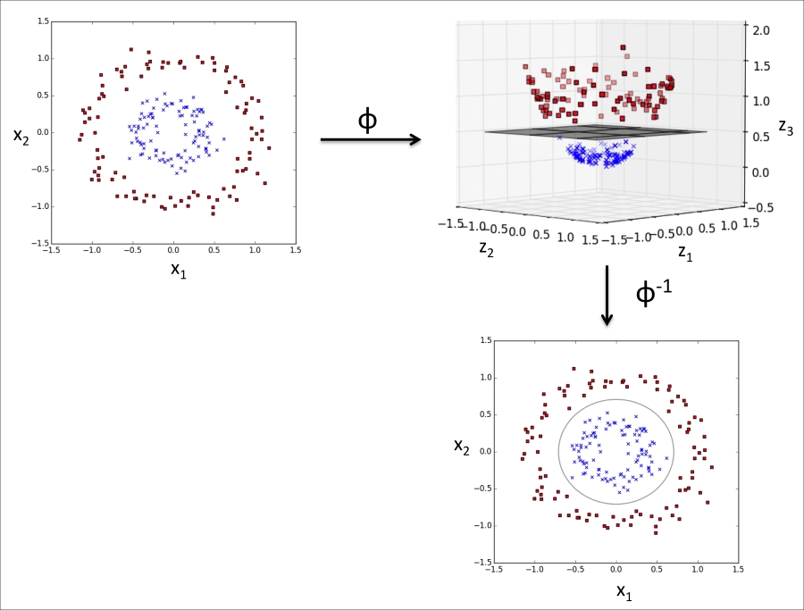
The basic idea behind kernel methods to deal with such linearly inseparable data is to create nonlinear combinations of the original features to project them onto a higher dimensional space via a mapping function ![]() where it becomes linearly separable. As shown in the next figure, we can transform a two-dimensional dataset onto a new three-dimensional feature space where the classes become separable via the following projection:
where it becomes linearly separable. As shown in the next figure, we can transform a two-dimensional dataset onto a new three-dimensional feature space where the classes become separable via the following projection:
This allows us to separate the two classes shown in the plot via a linear hyperplane that becomes a nonlinear decision boundary if we project it back onto the original feature space:
To solve a nonlinear problem using an SVM, we transform the training data onto a higher dimensional feature space via a mapping function ![]() and train a linear SVM model to classify the data in this new feature space. Then we can use the same mapping function
and train a linear SVM model to classify the data in this new feature space. Then we can use the same mapping function ![]() to transform new, unseen data to classify it using the linear SVM model.
to transform new, unseen data to classify it using the linear SVM model.
However, one problem with this mapping approach is that the construction of the new features is computationally very expensive, especially if we are dealing with high-dimensional data. This is where the so-called kernel trick comes into play. Although we didn't go into much detail about how to solve the quadratic programming task to train an SVM, in practice all we need is to replace the dot product ![]() by
by ![]() . In order to save the expensive step of calculating this dot product between two points explicitly, we define a so-called kernel function:
. In order to save the expensive step of calculating this dot product between two points explicitly, we define a so-called kernel function: ![]() =
= ![]() .
.
One of the most widely used kernels is the Radial Basis Function kernel (RBF kernel) or Gaussian kernel:

This is often simplified to:

Here,  is a free parameter that is to be optimized.
Roughly speaking, the term kernel can be interpreted as a similarity function between a pair of samples. The minus sign inverts the distance measure into a similarity score and, due to the exponential term, the resulting similarity score will fall into a range between 1 (for exactly similar samples) and 0 (for very dissimilar samples).
Now that we defined the big picture behind the kernel trick, let's see if we can train a kernel SVM that is able to draw a nonlinear decision boundary that separates the XOR data well. Here, we simply use the SVC class from scikit-learn that we imported earlier and replace the parameter kernel='linear' with kernel='rbf':
>>> svm = SVC(kernel='rbf', random_state=0, gamma=0.10, C=10.0)
>>> svm.fit(X_xor, y_xor)
>>> plot_decision_regions(X_xor, y_xor, classifier=svm)
>>> plt.legend(loc='upper left')
>>> plt.show()
As we can see in the resulting plot, the kernel SVM separates the XOR data relatively well:

The ![]() parameter, which we set to
parameter, which we set to gamma=0.1, can be understood as a cut-off parameter for the Gaussian sphere. If we increase the value for ![]() , we increase the influence or reach of the training samples, which leads to a softer decision boundary. To get a better intuition for
, we increase the influence or reach of the training samples, which leads to a softer decision boundary. To get a better intuition for ![]() , let's apply RBF kernel SVM to our Iris flower dataset:
, let's apply RBF kernel SVM to our Iris flower dataset:
>>> svm = SVC(kernel='rbf', random_state=0, gamma=0.2, C=1.0)
>>> svm.fit(X_train_std, y_train)
>>> plot_decision_regions(X_combined_std,
...                       y_combined, classifier=svm,
...                       test_idx=range(105,150))
>>> plt.xlabel('petal length [standardized]')
>>> plt.ylabel('petal width [standardized]')
>>> plt.legend(loc='upper left')
>>> plt.show()
Since we chose a relatively small value for ![]() , the resulting decision boundary of the RBF kernel SVM model will be relatively soft, as shown in the following figure:
, the resulting decision boundary of the RBF kernel SVM model will be relatively soft, as shown in the following figure:

Now let's increase the value of ![]() and observe the effect on the decision boundary:
and observe the effect on the decision boundary:
>>> svm = SVC(kernel='rbf', random_state=0, gamma=100.0, C=1.0)
>>> svm.fit(X_train_std, y_train)
>>> plot_decision_regions(X_combined_std,
...                       y_combined, classifier=svm,
...                       test_idx=range(105,150))
>>> plt.xlabel('petal length [standardized]')
>>> plt.ylabel('petal width [standardized]')
>>> plt.legend(loc='upper left')
>>> plt.show()
In the resulting plot, we can now see that the decision boundary around the classes 0 and 1 is much tighter using a relatively large value of ![]() :
:

Although the model fits the training dataset very well, such a classifier will likely have a high generalization error on unseen data, which illustrates that the optimization of ![]() also plays an important role in controlling overfitting.
also plays an important role in controlling overfitting.