
Many machine learning algorithms make assumptions about the linear separability of the input data. You learned that the perceptron even requires perfectly linearly separable training data to converge. Other algorithms that we have covered so far assume that the lack of perfect linear separability is due to noise: Adaline, logistic regression, and the (standard) support vector machine (SVM) to just name a few. However, if we are dealing with nonlinear problems, which we may encounter rather frequently in real-world applications, linear transformation techniques for dimensionality reduction, such as PCA and LDA, may not be the best choice. In this section, we will take a look at a kernelized version of PCA, or kernel PCA, which relates to the concepts of kernel SVM that we remember from Chapter 3, A Tour of Machine Learning Classifiers Using Scikit-learn. Using kernel PCA, we will learn how to transform data that is not linearly separable onto a new, lower-dimensional subspace that is suitable for linear classifiers.

As we remember from our discussion about kernel SVMs in Chapter 3, A Tour of Machine Learning Classifiers Using Scikit-learn, we can tackle nonlinear problems by projecting them onto a new feature space of higher dimensionality where the classes become linearly separable. To transform the samples ![]() onto this higher
onto this higher ![]() -dimensional subspace, we defined a nonlinear mapping function
-dimensional subspace, we defined a nonlinear mapping function ![]() :
:
We can think of ![]() as a function that creates nonlinear combinations of the original features to map the original
as a function that creates nonlinear combinations of the original features to map the original ![]() -dimensional dataset onto a larger,
-dimensional dataset onto a larger, ![]() -dimensional feature space. For example, if we had feature vector
-dimensional feature space. For example, if we had feature vector ![]() (
(![]() is a column vector consisting of
is a column vector consisting of ![]() features) with two dimensions
features) with two dimensions ![]() , a potential mapping onto a 3D space could be as follows:
, a potential mapping onto a 3D space could be as follows:
In other words, via kernel PCA we perform a nonlinear mapping that transforms the data onto a higher-dimensional space and use standard PCA in this higher-dimensional space to project the data back onto a lower-dimensional space where the samples can be separated by a linear classifier (under the condition that the samples can be separated by density in the input space). However, one downside of this approach is that it is computationally very expensive, and this is where we use the kernel trick. Using the kernel trick, we can compute the similarity between two high-dimension feature vectors in the original feature space.
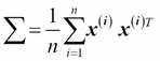
Before we proceed with more details about using the kernel trick to tackle this computationally expensive problem, let's look back at the standard PCA approach that we implemented at the beginning of this chapter. We computed the covariance between two features ![]() and
and ![]() as follows:
as follows:

Since the standardizing of features centers them at mean zero, for instance, ![]() and
and ![]() , we can simplify this equation as follows:
, we can simplify this equation as follows:

Note that the preceding equation refers to the covariance between two features; now, let's write the general equation to calculate the covariance matrix ![]() :
:
Bernhard Scholkopf generalized this approach (B. Scholkopf, A. Smola, and K.-R. Muller. Kernel Principal Component Analysis. pages 583–588, 1997) so that we can replace the dot products between samples in the original feature space by the nonlinear feature combinations via ![]() :
:

To obtain the eigenvectors—the principal components—from this covariance matrix, we have to solve the following equation:


Here, ![]() and
and ![]() are the eigenvalues and eigenvectors of the covariance matrix
are the eigenvalues and eigenvectors of the covariance matrix ![]() , and
, and ![]() can be obtained by extracting the eigenvectors of the kernel (similarity) matrix
can be obtained by extracting the eigenvectors of the kernel (similarity) matrix ![]() as we will see in the following paragraphs.
as we will see in the following paragraphs.
The derivation of the kernel matrix is as follows:
First, let's write the covariance matrix as in matrix notation, where ![]() is an
is an ![]() -dimensional matrix:
-dimensional matrix:

Now, we can write the eigenvector equation as follows:

Since ![]() , we get:
, we get:

Multiplying it by ![]() on both sides yields the following result:
on both sides yields the following result:


Here, ![]() is the similarity (kernel) matrix:
is the similarity (kernel) matrix:
As we recall from the SVM section in Chapter 3, A Tour of Machine Learning Classifiers Using Scikit-learn, we use the kernel trick to avoid calculating the pairwise dot products of the samples ![]() under
under ![]() explicitly by using a kernel function
explicitly by using a kernel function ![]() so that we don't need to calculate the eigenvectors explicitly:
so that we don't need to calculate the eigenvectors explicitly:
In other words, what we obtain after kernel PCA are the samples already projected onto the respective components rather than constructing a transformation matrix as in the standard PCA approach. Basically, the kernel function (or simply kernel) can be understood as a function that calculates a dot product between two vectors—a measure of similarity.
The most commonly used kernels are as follows:


To summarize what we have discussed so far, we can define the following three steps to implement an RBF kernel PCA:
-
We compute the kernel (similarity) matrix
 , where we need to calculate the following:
We do this for each pair of samples:
, where we need to calculate the following:
We do this for each pair of samples:

For example, if our dataset contains 100 training samples, the symmetric kernel matrix of the pair-wise similarities would be
 dimensional.
 -
We center the kernel matrix using the following equation:
Here,

 is an
is an  - dimensional matrix (the same dimensions as the kernel matrix) where all values are equal to
  .
.
-
We collect the top
 eigenvectors of the centered kernel matrix based on their corresponding eigenvalues, which are ranked by decreasing magnitude. In contrast to standard PCA, the eigenvectors are not the principal component axes but the samples projected onto those axes.
At this point, you may be wondering why we need to center the kernel matrix in the second step. We previously assumed that we are working with standardized data, where all features have mean zero when we formulated the covariance matrix and replaced the dot products by the nonlinear feature combinations via ![]() . Thus, the centering of the kernel matrix in the second step becomes necessary, since we do not compute the new feature space explicitly and we cannot guarantee that the new feature space is also centered at zero.
. Thus, the centering of the kernel matrix in the second step becomes necessary, since we do not compute the new feature space explicitly and we cannot guarantee that the new feature space is also centered at zero.
In the next section, we will put those three steps into action by implementing a kernel PCA in Python.
In the previous subsection, we discussed the core concepts behind kernel PCA. Now, we are going to implement an RBF kernel PCA in Python following the three steps that summarized the kernel PCA approach. Using the SciPy and NumPy helper functions, we will see that implementing a kernel PCA is actually really simple:
from scipy.spatial.distance import pdist, squareform
from scipy import exp
from scipy.linalg import eigh
import numpy as np

def rbf_kernel_pca(X, gamma, n_components):
    """
    RBF kernel PCA implementation.

    Parameters
    ------------
    X: {NumPy ndarray}, shape = [n_samples, n_features]

    gamma: float
      Tuning parameter of the RBF kernel

    n_components: int
      Number of principal components to return

    Returns
    ------------
     X_pc: {NumPy ndarray}, shape = [n_samples, k_features]
       Projected dataset

    """
    # Calculate pairwise squared Euclidean distances
    # in the MxN dimensional dataset.
    sq_dists = pdist(X, 'sqeuclidean')

    # Convert pairwise distances into a square matrix.
    mat_sq_dists = squareform(sq_dists)

    # Compute the symmetric kernel matrix.
    K = exp(-gamma * mat_sq_dists)

    # Center the kernel matrix.
    N = K.shape[0]
    one_n = np.ones((N,N)) / N
    K = K - one_n.dot(K) - K.dot(one_n) + one_n.dot(K).dot(one_n)

    # Obtaining eigenpairs from the centered kernel matrix
    # numpy.eigh returns them in sorted order
    eigvals, eigvecs = eigh(K)

    # Collect the top k eigenvectors (projected samples)
    X_pc = np.column_stack((eigvecs[:, -i]
                            for i in range(1, n_components + 1)))

    return X_pc
One downside of using an RBF kernel PCA for dimensionality reduction is that we have to specify the parameter ![]() a priori. Finding an appropriate value for
a priori. Finding an appropriate value for ![]() requires experimentation and is best done using algorithms for parameter tuning, for example, grid search, which we will discuss in more detail in Chapter 6, Learning Best Practices for Model Evaluation and Hyperparameter Tuning.
requires experimentation and is best done using algorithms for parameter tuning, for example, grid search, which we will discuss in more detail in Chapter 6, Learning Best Practices for Model Evaluation and Hyperparameter Tuning.
Now, let's apply our rbf_kernel_pca on some nonlinear example datasets. We will start by creating a two-dimensional dataset of 100 sample points representing two half-moon shapes:
>>> from sklearn.datasets import make_moons
>>> X, y = make_moons(n_samples=100, random_state=123)
>>> plt.scatter(X[y==0, 0], X[y==0, 1],
...             color='red', marker='^', alpha=0.5)
>>> plt.scatter(X[y==1, 0], X[y==1, 1],
...             color='blue', marker='o', alpha=0.5)
>>> plt.show()
For the purposes of illustration, the half-moon of triangular symbols shall represent one class and the half-moon depicted by the circular symbols represent the samples from another class:

Clearly, these two half-moon shapes are not linearly separable and our goal is to unfold the half-moons via kernel PCA so that the dataset can serve as a suitable input for a linear classifier. But first, let's see what the dataset looks like if we project it onto the principal components via standard PCA:
>>> from sklearn.decomposition import PCA
>>> scikit_pca = PCA(n_components=2)
>>> X_spca = scikit_pca.fit_transform(X)
>>> fig, ax = plt.subplots(nrows=1,ncols=2, figsize=(7,3))
>>> ax[0].scatter(X_spca[y==0, 0], X_spca[y==0, 1],
...               color='red', marker='^', alpha=0.5)
>>> ax[0].scatter(X_spca[y==1, 0], X_spca[y==1, 1],
...               color='blue', marker='o', alpha=0.5)
>>> ax[1].scatter(X_spca[y==0, 0], np.zeros((50,1))+0.02,
...               color='red', marker='^', alpha=0.5)
>>> ax[1].scatter(X_spca[y==1, 0], np.zeros((50,1))-0.02,
...               color='blue', marker='o', alpha=0.5)
>>> ax[0].set_xlabel('PC1')
>>> ax[0].set_ylabel('PC2')
>>> ax[1].set_ylim([-1, 1])
>>> ax[1].set_yticks([])
>>> ax[1].set_xlabel('PC1')
>>> plt.show()
Clearly, we can see in the resulting figure that a linear classifier would be unable to perform well on the dataset transformed via standard PCA:

Note that when we plotted the first principal component only (right subplot), we shifted the triangular samples slightly upwards and the circular samples slightly downwards to better visualize the class overlap.
Now, let's try out our kernel PCA function rbf_kernel_pca, which we implemented in the previous subsection:
>>> from matplotlib.ticker import FormatStrFormatter
>>> X_kpca = rbf_kernel_pca(X, gamma=15, n_components=2)
>>> fig, ax = plt.subplots(nrows=1,ncols=2, figsize=(7,3))
>>> ax[0].scatter(X_kpca[y==0, 0], X_kpca[y==0, 1],
...               color='red', marker='^', alpha=0.5)
>>> ax[0].scatter(X_kpca[y==1, 0], X_kpca[y==1, 1],
...               color='blue', marker='o', alpha=0.5)
>>> ax[1].scatter(X_kpca[y==0, 0], np.zeros((50,1))+0.02,
...               color='red', marker='^', alpha=0.5)
>>> ax[1].scatter(X_kpca[y==1, 0], np.zeros((50,1))-0.02,
...               color='blue', marker='o', alpha=0.5)
>>> ax[0].set_xlabel('PC1')
>>> ax[0].set_ylabel('PC2')
>>> ax[1].set_ylim([-1, 1])
>>> ax[1].set_yticks([])
>>> ax[1].set_xlabel('PC1')
>>> ax[0].xaxis.set_major_formatter(FormatStrFormatter('%0.1f'))
>>> ax[1].xaxis.set_major_formatter(FormatStrFormatter('%0.1f'))
>>> plt.show()
We can now see that the two classes (circles and triangles) are linearly well separated so that it becomes a suitable training dataset for linear classifiers:

Unfortunately, there is no universal value for the tuning parameter ![]() that works well for different datasets. To find a
that works well for different datasets. To find a ![]() value that is appropriate for a given problem requires experimentation. In Chapter 6, Learning Best Practices for Model Evaluation and Hyperparameter Tuning, we will discuss techniques that can help us to automate the task of optimizing such tuning parameters. Here, I will use values for
value that is appropriate for a given problem requires experimentation. In Chapter 6, Learning Best Practices for Model Evaluation and Hyperparameter Tuning, we will discuss techniques that can help us to automate the task of optimizing such tuning parameters. Here, I will use values for ![]() that I found produce good results.
that I found produce good results.
In the previous subsection, we showed you how to separate half-moon shapes via kernel PCA. Since we put so much effort into understanding the concepts of kernel PCA, let's take a look at another interesting example of a nonlinear problem: concentric circles.
The code is as follows:
>>> from sklearn.datasets import make_circles
>>> X, y = make_circles(n_samples=1000,
...            random_state=123, noise=0.1, factor=0.2)
>>> plt.scatter(X[y==0, 0], X[y==0, 1],
...            color='red', marker='^', alpha=0.5)
>>> plt.scatter(X[y==1, 0], X[y==1, 1],
...            color='blue', marker='o', alpha=0.5)
>>> plt.show()
Again, we assume a two-class problem where the triangle shapes represent one class and the circle shapes represent another class, respectively:

Let's start with the standard PCA approach to compare it with the results of the RBF kernel PCA:
>>> scikit_pca = PCA(n_components=2)
>>> X_spca = scikit_pca.fit_transform(X)
>>> fig, ax = plt.subplots(nrows=1,ncols=2, figsize=(7,3))
>>> ax[0].scatter(X_spca[y==0, 0], X_spca[y==0, 1],
...               color='red', marker='^', alpha=0.5)
>>> ax[0].scatter(X_spca[y==1, 0], X_spca[y==1, 1],
...               color='blue', marker='o', alpha=0.5)
>>> ax[1].scatter(X_spca[y==0, 0], np.zeros((500,1))+0.02,
...              color='red', marker='^', alpha=0.5)
>>> ax[1].scatter(X_spca[y==1, 0], np.zeros((500,1))-0.02,
...               color='blue', marker='o', alpha=0.5)
>>> ax[0].set_xlabel('PC1')
>>> ax[0].set_ylabel('PC2')
>>> ax[1].set_ylim([-1, 1])
>>> ax[1].set_yticks([])
>>> ax[1].set_xlabel('PC1')
>>> plt.show()
Again, we can see that standard PCA is not able to produce results suitable for training a linear classifier:

Given an appropriate value for ![]() , let's see if we are luckier using the RBF kernel PCA implementation:
, let's see if we are luckier using the RBF kernel PCA implementation:
>>> X_kpca = rbf_kernel_pca(X, gamma=15, n_components=2)
>>> fig, ax = plt.subplots(nrows=1,ncols=2, figsize=(7,3))
>>> ax[0].scatter(X_kpca[y==0, 0], X_kpca[y==0, 1],
...               color='red', marker='^', alpha=0.5)
>>> ax[0].scatter(X_kpca[y==1, 0], X_kpca[y==1, 1],
...               color='blue', marker='o', alpha=0.5)
>>> ax[1].scatter(X_kpca[y==0, 0], np.zeros((500,1))+0.02,
...               color='red', marker='^', alpha=0.5)
>>> ax[1].scatter(X_kpca[y==1, 0], np.zeros((500,1))-0.02,
...               color='blue', marker='o', alpha=0.5)
>>> ax[0].set_xlabel('PC1')
>>> ax[0].set_ylabel('PC2')
>>> ax[1].set_ylim([-1, 1])
>>> ax[1].set_yticks([])
>>> ax[1].set_xlabel('PC1')
>>> plt.show()
Again, the RBF kernel PCA projected the data onto a new subspace where the two classes become linearly separable:

In the two previous example applications of kernel PCA, the half-moon shapes and the concentric circles, we projected a single dataset onto a new feature. In real applications, however, we may have more than one dataset that we want to transform, for example, training and test data, and typically also new samples we will collect after the model building and evaluation. In this section, you will learn how to project data points that were not part of the training dataset.
As we remember from the standard PCA approach at the beginning of this chapter, we project data by calculating the dot product between a transformation matrix and the input samples; the columns of the projection matrix are the top ![]() eigenvectors (
eigenvectors (![]() ) that we obtained from the covariance matrix. Now, the question is how can we transfer this concept to kernel PCA? If we think back to the idea behind kernel PCA, we remember that we obtained an eigenvector (
) that we obtained from the covariance matrix. Now, the question is how can we transfer this concept to kernel PCA? If we think back to the idea behind kernel PCA, we remember that we obtained an eigenvector (![]() ) of the centered kernel matrix (not the covariance matrix), which means that those are the samples that are already projected onto the principal component axis
) of the centered kernel matrix (not the covariance matrix), which means that those are the samples that are already projected onto the principal component axis ![]() . Thus, if we want to project a new sample
. Thus, if we want to project a new sample ![]() onto this principal component axis, we'd need to compute the following:
onto this principal component axis, we'd need to compute the following:
Fortunately, we can use the kernel trick so that we don't have to calculate the projection ![]() explicitly. However, it is worth noting that kernel PCA, in contrast to standard PCA, is a memory-based method, which means that we have to reuse the original training set each time to project new samples. We have to calculate the pairwise RBF kernel (similarity) between each
explicitly. However, it is worth noting that kernel PCA, in contrast to standard PCA, is a memory-based method, which means that we have to reuse the original training set each time to project new samples. We have to calculate the pairwise RBF kernel (similarity) between each ![]() th sample in the training dataset and the new sample
th sample in the training dataset and the new sample ![]() :
:

Here, eigenvectors ![]() and eigenvalues
and eigenvalues ![]() of the Kernel matrix
of the Kernel matrix ![]() satisfy the following condition in the equation:
satisfy the following condition in the equation:
After calculating the similarity between the new samples and the samples in the training set, we have to normalize the eigenvector ![]() by its eigenvalue. Thus, let's modify the
by its eigenvalue. Thus, let's modify the rbf_kernel_pca function that we implemented earlier so that it also returns the eigenvalues of the kernel matrix:
from scipy.spatial.distance import pdist, squareform
from scipy import exp
from scipy.linalg import eigh
import numpy as np

def rbf_kernel_pca(X, gamma, n_components):
    """
    RBF kernel PCA implementation.

    Parameters
    ------------
    X: {NumPy ndarray}, shape = [n_samples, n_features]

    gamma: float
      Tuning parameter of the RBF kernel

    n_components: int
      Number of principal components to return

    Returns
    ------------
     X_pc: {NumPy ndarray}, shape = [n_samples, k_features]
       Projected dataset

     lambdas: list
       Eigenvalues

    """
    # Calculate pairwise squared Euclidean distances
    # in the MxN dimensional dataset.
    sq_dists = pdist(X, 'sqeuclidean')

    # Convert pairwise distances into a square matrix.
    mat_sq_dists = squareform(sq_dists)

    # Compute the symmetric kernel matrix.
    K = exp(-gamma * mat_sq_dists)

    # Center the kernel matrix.
    N = K.shape[0]
    one_n = np.ones((N,N)) / N
    K = K - one_n.dot(K) - K.dot(one_n) + one_n.dot(K).dot(one_n)

    # Obtaining eigenpairs from the centered kernel matrix
    # numpy.eigh returns them in sorted order
    eigvals, eigvecs = eigh(K)

    # Collect the top k eigenvectors (projected samples)
    alphas = np.column_stack((eigvecs[:,-i]
                    for i in range(1,n_components+1)))

    # Collect the corresponding eigenvalues
    lambdas = [eigvals[-i] for i in range(1,n_components+1)]

    return alphas, lambdas
Now, let's create a new half-moon dataset and project it onto a one-dimensional subspace using the updated RBF kernel PCA implementation:
>>> X, y = make_moons(n_samples=100, random_state=123)
>>> alphas, lambdas =rbf_kernel_pca(X, gamma=15, n_components=1)
To make sure that we implement the code for projecting new samples, let's assume that the 26th point from the half-moon dataset is a new data point ![]() , and our task is to project it onto this new subspace:
, and our task is to project it onto this new subspace:
>>> x_new = X[25]
>>> x_new
array([ 1.8713187 ,  0.00928245])
>>> x_proj = alphas[25] # original projection
>>> x_proj
array([ 0.07877284])
>>> def project_x(x_new, X, gamma, alphas, lambdas):
...     pair_dist = np.array([np.sum(
...                  (x_new-row)**2) for row in X])
...     k = np.exp(-gamma * pair_dist)
... return k.dot(alphas / lambdas)
By executing the following code, we are able to reproduce the original projection. Using the project_x function, we will be able to project any new data samples as well. The code is as follows:
>>> x_reproj = project_x(x_new, X,
...       gamma=15, alphas=alphas, lambdas=lambdas)
>>> x_reproj
array([ 0.07877284])
Lastly, let's visualize the projection on the first principal component:
>>> plt.scatter(alphas[y==0, 0], np.zeros((50)),
...             color='red', marker='^',alpha=0.5)
>>> plt.scatter(alphas[y==1, 0], np.zeros((50)),
...             color='blue', marker='o', alpha=0.5)
>>> plt.scatter(x_proj, 0, color='black',
...             label='original projection of point X[25]',
...             marker='^', s=100)
>>> plt.scatter(x_reproj, 0, color='green',
...             label='remapped point X[25]',
...             marker='x', s=500)
>>> plt.legend(scatterpoints=1)
>>> plt.show()
As we can see in the following scatterplot, we mapped the sample ![]() onto the first principal component correctly:
onto the first principal component correctly:

For our convenience, scikit-learn implements a kernel PCA class in the sklearn.decomposition submodule. The usage is similar to the standard PCA class, and we can specify the kernel via the kernel parameter:
>>> from sklearn.decomposition import KernelPCA
>>> X, y = make_moons(n_samples=100, random_state=123)
>>> scikit_kpca = KernelPCA(n_components=2,
...               kernel='rbf', gamma=15)
>>> X_skernpca = scikit_kpca.fit_transform(X)
To see if we get results that are consistent with our own kernel PCA implementation, let's plot the transformed half-moon shape data onto the first two principal components:
>>> plt.scatter(X_skernpca[y==0, 0], X_skernpca[y==0, 1],
...             color='red', marker='^', alpha=0.5)
>>> plt.scatter(X_skernpca[y==1, 0], X_skernpca[y==1, 1],
...             color='blue', marker='o', alpha=0.5)
>>> plt.xlabel('PC1')
>>> plt.ylabel('PC2')
>>> plt.show()
As we can see, the results of the scikit-learn KernelPCA are consistent with our own implementation:

Note
Scikit-learn also implements advanced techniques for nonlinear dimensionality reduction that are beyond the scope of this book. You can find a nice overview of the current implementations in scikit-learn complemented with illustrative examples at http://scikit-learn.org/stable/modules/manifold.html.


