4. Single-Dielectric Configurations

Search in book...
Toggle Font Controls
Create new playlist

Name your new playlist

Playlist description (optional)
Sign In

Email address

Password

Forgot Password?

or

Continue with Facebook

Continue with Google
Sign Up

Full Name

Email address

Confirm Email Address

Password

or

Continue with Facebook

Continue with Google

ABSTRACT Although most of the real-life configurations are multi-dielectric in nature, it is required to study some of the single-dielectric arrangements, which are commonly used, for the proper understanding of the application of theory in determining electric field in practical cases. This chapter presents a physical explanation of displacement current and also discusses in details the energy stored in an electric field. Three single-dielectric arrangements are analyzed and how such analysis can be used for most economical use of insulating materials has also been discussed with the help of state-of-the-art examples.

4.1 Introduction

Mother Nature has presented the humankind an insulation as a gift, which is available in abundance and is also free. This dielectric is nothing but the atmospheric air. It is not difficult to conceive that no electrical system would have worked had air been not an insulating medium. Because air is present everywhere, most of the real-life arrangements are multi-dielectric configurations where the equipment insulation, whether it is solid, liquid or gaseous or a combination of two or more of these insulating media, is commonly surrounded by atmospheric air. However, there are specific cases where the configuration could be single-dielectric one, for example, a co-axial cable having only one dielectric medium. Analysis of single-dielectric arrangement is necessary to grasp the theoretical aspects of electric field in a meaningful way. Moreover, there are certain aspects such as displacement current and energy stored in an electric field, which need to be understood from a single-dielectric viewpoint to start with.

4.2 Displacement Current

Consider a capacitor with a perfect dielectric or, say vacuum, in between its two plates. In such a case, no charge can move through the perfect dielectric or vacuum. In other words, there could be no current flowing between the two plates within the capacitor. Now if a DC voltage is applied between its two plates, then a charging current flows from the source to supply the charges to the plates of the capacitor for a short duration of charging. When the capacitor is fully charged, the charging current ceases to flow. It is to be noted here that this charging current is measurable only in the circuit between the source and the capacitor. If one tries to measure the current between the plates within the capacitor, then the result of the current measurement will be zero. It means that this charging current does not flow through the entire closed loop formed by the source and the capacitor. But why these charges are to be supplied by the source to the capacitor plates? The answer is that the capacitor with a perfect dielectric or vacuum is an open circuit and hence the potential difference between the capacitor plates will be equal to the source voltage. Accordingly, there will be an electric field established between the capacitor plates. In order to establish this electric field, charges have to be supplied from the source to the capacitor plates.

Depending on the area and separation distance between the plates, there is a finite capacitance of the capacitor. Hence, if an AC voltage is applied between the plates of the capacitor, a capacitive current will flow in the circuit, which will be a continuous current varying with time that could be measured by an ammeter placed in between the source and the capacitor. However, due to perfect dielectric or vacuum, as stated earlier, there could be no movement of charge between the plates within the capacitor. Hence, this continuous capacitive current is measurable only in the circuit between the AC source and the capacitor plates. Then the question is how this continuous capacitive current appears in a section of the circuit external to the capacitor plates and not through the whole circuit? The answer to this question lies in the fact that this current is not conduction current. It appears due to the displacement of charges between the source and the capacitor plates, even when there is no charge movement between the plates within the capacitor. Consequently, this current is termed as displacement current. The concept of displacement current may be explained as detailed below.

Images

FIGURE 4.1
Physical explanation of the displacement current of a capacitor.

Take the example of a capacitor with vacuum between its plates, as shown in Figure 4.1. If the separation distance between the plates is much smaller than the plate length/diameter and if fringing of flux at the edges is neglected, then the electric field between the capacitor plates will be uniform. If the potential difference between its plates at any time instant is v and the separation distance between the plates is d, then the magnitude of electric field intensity between the capacitor plates at that time instant will be (v/d). Thus, a unit positive charge placed in vacuum between the plates within the capacitor will experience this force on the unit change due to the charges present on the capacitor plates. Owing to the application of alternating voltage, the electric field intensity within the capacitor (= v/d) will vary in direct proportion to the potential difference between the plates. Consequently, for this variation in electric field intensity, the amount of charge on the capacitor plates will again have to vary in direct proportion to the potential difference between the plates. Let the amount of charge on the capacitor plates corresponding to the peak value (V_m) of the sinusoidal applied voltage be q_m.

At θ = 0°, the potential difference across the capacitor plates is zero and hence the charge on the plates is also zero, as shown in Figure 4.1a. Then the charge on the plates increases with time as the sinusoidal voltage magnitude increases with time from θ = 0° to θ = 90°, as shown in Figure 4.1a–c. These charges are supplied by the AC source to the capacitor plates and hence in the circuit between the source and the capacitor plates, there is a change in charge with time (dq/dt). Whenever there is such change in charge with time, there is a measurable current. Therefore, if an ammeter is placed in between the source and the capacitor, this current can be measured. The magnitude of this current will be determined by the rate of change of charge, which is the same as the rate of change of voltage with time, as explained earlier in this section. As shown in Figure 4.2, the rate of change of sinusoidal voltage is maximum at the zero crossing of the voltage waveform, that is, at θ = 0°, and is zero at the voltage peak, that is, at θ = 90°. In between this time span, this current will also have a sinusoidal variation with time.

Images

FIGURE 4.2
Slope of sinusoidal voltage waveform.

From θ = 90° to θ = 180°, the negative slope of sinusoidal voltage waveform increases from zero to maximum at the voltage zero crossing at θ = 180°. The magnitude of voltage starts decreasing from θ = 90° and hence the charges on the capacitor plates also start decreasing from q_m corresponding to θ = 90°. In other words, the charges start to move from the capacitor plate back to the source. Hence, the ammeter between the source and the capacitor will record a current in the opposite direction, which will increase in magnitude from θ = 90° and will become maximum at θ = 180° in this opposite direction. The same sequential process will be repeated from θ = 180° to θ = 360° albeit the direction will be just the opposite of that between θ = 0° and θ = 90°.

Therefore, it could be seen that although there is no charge movement between the plates within the capacitor itself, there is a continuous displacement of charges between the source and the capacitor plates in the external circuit. As a result, the displacement current flows in the external circuit. From the above discussion, it can be noted that (1) the current is positive maximum when dq/dt and consequently dv/dt is positive maximum at θ = 0°; (2) the current is zero when dq/dt and consequently dv/dt is zero when θ = 90°; (3) the current is at its negative maximum when dq/dt and consequently dv/dt is at its negative maximum at θ = 180° and so on. Considering the facts from (1) to (3), it can be concluded that there is a phase difference of 90° between the potential across the capacitor plates and the displacement current, and this displacement current leads the potential by 90°.

In real life, the dielectric between the capacitor plates is never a perfect one and hence a small amount of conduction current flows between the capacitor plates. Consequently, the current through a real-life capacitor leads the potential by an angle slightly less than 90°.

4.3 Parallel Plate Capacitor

A capacitor is an arrangement of conductors along with dielectrics that is used primarily to store electric charge. A very simple capacitor is a system consisting of two parallel metallic plates with free space or any dielectric in between, as shown in Figure 4.3.

Images

FIGURE 4.3
Parallel plate capacitor arrangement.

Images

FIGURE 4.4
Field due to infinitely long-charged sheet.

In order to understand the electric field within a parallel plate capacitor, it is necessary to know the electric field due to infinitely long-charged planar sheet having uniform surface charge density (σ). As an infinitely long plane possesses a planar symmetry and the charge is uniformly distributed on the planar surface, the electric field intensity acts in the direction of the normal to the plane. In other words, the magnitude of the electric field intensity is constant on all the planes that are parallel to the charged sheet.

To analyze the field due to such a charged sheet, the best choice for a Gaussian surface is a cylinder whose axis is perpendicular to the plane, as shown in Figure 4.4. As the surface charge density is assumed to be uniform, the charge enclosed by the Gaussian surface is given by (σA). As shown in Figure 4.4, the electric field intensity vector is parallel to the area vector at the two end surfaces and is normal to the area vector on the curved wall surfaces. Hence, applying Gauss’s law on the cylindrical Gaussian surface

$\int_{Cylinder surface} ε_{0} \vec{E} \cdot d \vec{A} = σ A$

$\begin{matrix} or, ε_{0} \int_{Walls} | \vec{E} | \cos (9 0^{o}) d A + 2 ε_{0} \int_{Ends} | \vec{E} | \cos (0^{o}) d A = σ A \\ or, 0 + 2 ε_{0} | \vec{E} | A = σ A or, | \vec{E} | = \frac{σ}{2 ε_{0}} \end{matrix} (4.1)$

When two plates of equal and opposite charge density are placed near and parallel to each other with free space between them, the electric field intensities due to the two plates add between the plates while they cancel each other outside the plates, as shown in Figure 4.5. Thus, the electric field intensity between the two plates is given by E = σ/ε₀.

When the separation distance between the two plates is small compared to the sides of the plate, then the electric field intensity between the plates is constant throughout the interior of the capacitor. The flux lines are parallel to each other near the centre of the capacitor, whereas the concentration of flux lines occurs at the edges, which is known as fringing of flux, as shown in Figure 4.6. Neglecting fringing of flux and considering the potential difference between the two plates to be V, the electric field intensity can also be written as E = V/d.

Noting that the charge on the plates Q = σA, it may be written as follows:

$\frac{σ}{ε_{0}} = \frac{V}{d} or, \frac{Q A}{ε_{0}} = \frac{V}{d} or, \frac{Q}{V} = \frac{ε_{0} A}{d} or, C = \frac{ε_{0} A}{d} (4.2)$

where:

C is the capacitance of the parallel plate capacitor

Images

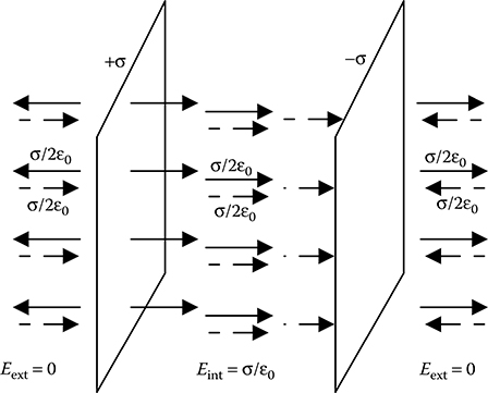
FIGURE 4.5
E-field within a parallel plate capacitor.

Images

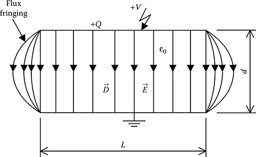
FIGURE 4.6
Flux lines in a parallel plate capacitor.

Equation 4.2 shows that the capacitance of a parallel capacitor is independent of the charge on the plates or the potential difference across the capacitor plates.

If any dielectric medium of relative permittivity (ε_r) is inserted between the plates, then the electric field intensity within the capacitor remains unchanged (= V/d), but the capacitance (C) is changed to (ε_rε₀A)/d.

4.3.1 Energy Stored in a Parallel Plate Capacitor

Consider that a parallel plate capacitor has no charge at the beginning. Now, if a voltage source is connected across its plates, so that the potential difference between the two plates becomes V, then the capacitor gets charged and these charges are supplied by the source to the capacitor plates. In order to supply these charges to the capacitor plates, some work have to be done by the external source, which is then stored as electrostatic energy in the capacitor.

Let, at any instant, the charge on the capacitor plates be +q and −q, respectively, and the potential difference between the plates is v. At this instant, consider that an additional amount of charge dq is supplied by the source to the plates. Then the energy spent by the source to deliver this charge is vdq and this energy is stored in the electric field of the capacitor.

Therefore, if the total charge on the plates are +Q and −Q, respectively, and the corresponding potential difference between the plates is V, then the total energy stored in the electric field is given by

$W = \int_{0}^{Q} v d q = \int_{0}^{Q} \frac{q}{C} d q = \frac{Q^{2}}{C} = \frac{C^{2} V^{2}}{2 C} = \frac{1}{2} C V^{2} (4.3)$

Now, surface charge density on the plates (σ) = (Q/A) = D. Therefore,

$W = \frac{Q^{2}}{2 C} = \frac{D^{2} A^{2}}{2 C} = \frac{ε^{2} E^{2} A^{2}}{2 (ε A / d)} = \frac{1}{2} ε E^{2} (A d)$

(Ad) being the volume of the parallel plate capacitor, the total energy stored in electric field per unit volume, that is, energy density, is given by

$W_{E} = \frac{1}{2} ε E^{2} (4.4)$

However, such a derivation for energy stored in electric field is only valid for a parallel plate capacitor. A more generalized way of obtaining the energy stored in the electric field is discussed in Section 4.4.

4.4 Energy Stored in Electric Field

Images

FIGURE 4.7
Assembling a set of charges.

Consider that an electric field is established by an assembly of charges. To obtain the energy stored in this electric field, the work done to assemble these charges need to be determined. Assume that all the charges are point charges, which are at infinity initially, and an external agent brings these charges one by one and places them at the respective positions, as shown in Figure 4.7. It is obvious that no work is to be done to bring the first charge q₁ from infinity to its location at P₁, as there is no existing electric field created by another charge. Then the second charge q₂ is brought from infinity to P₂ within the electric field created by q₁. Therefore, the work done in bringing the charge q₂ will be given by

$W_{2} = q_{2} ϕ_{21} = q_{2} \frac{q_{1}}{4 π ε_{0} r_{21}} (4.5)$

where:

ϕ₂₁ is the potential at the location P₂ due to the charge q₁ located at P₁

Then the third charge q₃ is brought from infinity to P₃ within the electric field created by q₁ and q₂. Therefore, the work done in bringing the charge q₃ will be given by

$W_{3} = q_{3} ϕ_{31} + q_{3} ϕ_{32} = q_{3} \frac{q_{1}}{4 π ε_{0} r_{31}} + q_{3} \frac{q_{2}}{4 π ε_{0} r_{32}} = \frac{1}{4 π ε_{0}} (\frac{q_{1} q_{3}}{r_{31}} + \frac{q_{2} q_{3}}{r_{32}}) (4.6)$

Therefore, the total work done in bringing q₁, q₂ and q₃ is as follows:

$0 + W_{2} + W_{3} = \frac{1}{4 π ε_{0}} (\frac{q_{1} q_{2}}{r_{21}} + \frac{q_{1} q_{3}}{r_{31}} + \frac{q_{2} q_{3}}{r_{32}}) (4.7)$

Denoting the charge that is being brought in by the suffix i and the charges that created the field within which this ith charge is being brought in by the suffix j, the work done in assembling N number of charges q₁, q₂, …, q_N can be written as follows:

$W = \sum_{i = 2}^{N} W^{r_{i}} = \frac{1}{4 π ε_{0}} \sum_{i = 2}^{N} \sum_{j = 1}^{i - 1} \frac{q_{i} q_{j}}{r_{i j}} (4.8)$

Figure 4.8 gives a pictorial representation of the numbers over which the summation of Equation 4.8 is being carried out. This summation is clearly over the triangular region marked I in Figure 4.8. Because the quantity being summed is symmetric in i and j, the same energy W would be obtained by a summation over the triangular region marked II in Figure 4.8. The summation over the triangular regions I and II must then give 2W. Thus W may also be obtained as follows:

$W' = \frac{1}{8 π ε_{0}} \sum_{i = 1}^{N} \sum_{j = 1}^{N} \frac{q_{i} q_{j}}{r_{i j}}, i \neq j (4.9)$

Instead of considering discrete point charges, if the charge distribution is taken as continuous throughout the volume V of Figure 4.7, then the potential at any point can be found by summing the contributions from individual differential volume elements of charge. Thus, by writing ρ(r)dV in place of q_i and ρ(r′)dV′ in place of q_j, the summation may be replaced by integrations over volume, which must be large enough to contain all the charges present. Thus, the work done to form a continuous charge distribution is given by

Images

FIGURE 4.8
Representation of summation to obtain energy stored.

$W = \frac{1}{8 π ε_{0}} \int_{V} \int_{V'} \frac{ρ (r) ρ (r')}{R_{r r'}} d V' d V (4.10)$

where:

$R_{r r'} = | r - \vec{r}' |$

The potential at the location r due to all the charges located at the respective positions r′ is given by

$ϕ (r) = \int_{V'} \frac{ρ (r')}{4 π ε_{0} R_{r r'}} d V' (4.11)$

Substitution of Equation 4.11 in Equation 4.10 yields

$W = \frac{1}{2} \int_{V} ρ (r) ϕ (r) d V (4.12)$

Because Equation 4.12 deals with quantities related to only one location r, the parameter r is omitted hereafter. Noting that $\vec{\nabla} . \vec{D} = ρ$ , Equation 4.12 could be rewritten as follows:

$W = \frac{1}{2} \int_{V} ϕ (\vec{\nabla} \cdot \vec{D}) d V (4.13)$

For any vector $\vec{D}$ and any scalar ϕ, the following vector identity could be written:

$\begin{matrix} \vec{\nabla} \cdot (ϕ \vec{D}) = \vec{D} \cdot \vec{\nabla} ϕ + ϕ (\vec{\nabla} \cdot \vec{D}) \\ or, ϕ (\vec{\nabla} \cdot \vec{D}) = \vec{\nabla} \cdot (ϕ \vec{D}) - \vec{D} \cdot \vec{\nabla} ϕ \end{matrix} (4.14)$

Therefore, from Equations 4.13 and 4.14,

$W = \frac{1}{2} \int_{V} \vec{\nabla} \cdot (ϕ \vec{D}) d V - \frac{1}{2} \int_{V} (\vec{D} \cdot \vec{\nabla} ϕ) d V (4.15)$

Applying divergence theorem to the first term on the right-hand side (RHS) of Equation 4.15,

$W = \frac{1}{2} \oint_{S} ϕ \vec{D} \cdot d \vec{S} - \frac{1}{2} \int_{V} (\vec{D} \cdot \vec{\nabla} ϕ) d V (4.16)$

As $\vec{E} = - \vec{\nabla} ϕ$ and $\vec{D} = ε_{0} \vec{E}$ , the above equation is rewritten as follows:

$W = \frac{1}{2} \oint_{s} ϕ \vec{D} \cdot d \vec{S} + \frac{1}{2} \int_{V} ε_{0} (\vec{E} \cdot \vec{E}) d V (4.17)$

In the first term on the RHS of Equation 4.17, ϕ varies as 1/r, whereas $\vec{D}$ varies as 1/r and surface term varies as r². Therefore, as a whole the first term varies as 1/r. If the bounding surface of volume V, as shown in Figure 4.7, is expanded from S to S₁, then the region between S and S₁ does not contribute to the energy integral, as there is no charge located in this region. However, although this region between S and S₁ is charge free, the electric field intensity is not zero in this region. Hence, as the bounding surface is expanded, the second term of Equation 4.17 will increase. Then, in order to keep the energy integral unchanged, the first term should decrease. Thus, if the bounding surface is taken to be infinitely large, then the first term on the RHS of Equation 4.17 becomes zero, keeping the total energy same. Therefore, the total work done in forming the continuous charge distribution, that is, the total energy stored in the electric field, is given by

$W = \frac{1}{2} \int_{V} ε_{0} E^{2} d V (4.18)$

Hence, energy stored per unit volume, that is, energy density, is given by

$W_{E} = \frac{1}{2} ε_{0} E^{2} (4.19)$

Considering the relative permittivity of the dielectric medium to be ε_r, energy density of an electric field is given by

$W_{E} = \frac{1}{2} ε_{r} ε_{0} E^{2} (4.20)$

Equation 4.20 is very useful in computing the energy stored in a complex dielectric arrangement where electric field intensity is non-uniform. In such cases, the electric field distribution is first determined using suitable method and then the entire volume under consideration is divided into smaller volume elements, so that each volume element contains only one dielectric medium and the electric field intensity remains constant within the volume element. As a result, the energy stored in each element can be computed using Equation 4.20. The energy stored in all the volume elements could then be summed up to get the total energy stored in any real-life dielectric arrangement having complex geometries and several dielectric media.

PROBLEM 4.1

Three point charges of magnitude −2, −3 and 1 nC are located in free space at (0,0,0)m, (0,2,0)m and (2,0,0)m, respectively. Find the energy stored in the system of charges.

Solution:

Denoting the charges as q₁ = −2 nC, q₂ = −3 nC and q₃ = 1 nC, no work is done to bring in q₁.

Electric potential at the location of q₂ due to q₁ is

$ϕ_{21} = \frac{- 2 \times 1 0^{- 9}}{4 \times π \times 8.8 54 \times 1 0^{- 12} \times r_{21}}$

where:

$r_{21} = \sqrt{0 + 2^{2} + 0} = 2 m$

Hence,

ϕ₂₁ = –8.987 V

Therefore, work done to bring in q₂ = −3 × 10⁻⁹×−8.987 = 26.96 nJ.

Again, electric potential at the location of q₃ due to q₁ is

$ϕ_{31} = \frac{- 2 \times 1 0^{- 9}}{4 \times π \times 8.8 54 \times 1 0^{- 12} \times r_{31}}$

where:

$r_{31} = \sqrt{0 + 0 + 2^{2}} = 2 m$

Hence,

ϕ₃₁ = –8.987 V

and electric potential at the location of q₃ due to q₂ is

$ϕ_{32} = \frac{- 3 \times 1 0^{- 9}}{4 \times π \times 8.8 54 \times 1 0^{- 12} \times r_{32}}$

where:

$r_{32} = \sqrt{0 + 2^{2} + 2^{2}} = 2 \sqrt{2} m$

Hence,

ϕ₃₂ = –6.354 V

Therefore, work done to bring in q₃ = 1 × 10⁻⁹ × (−8.987 − 6.354) = −15.34 nJ.

Hence, the total energy stored in the charge system = (26.96–15.34) = 11.62 nJ.

4.5 Two Concentric Spheres with Homogeneous Dielectric

A simple single-dielectric arrangement that have spherical symmetry is two concentric spheres with a homogeneous dielectric medium in between the two spheres, as shown in Figure 4.9. The inner sphere is charged to an electric potential +V, whereas the outer sphere is earthed.

Because this configuration has spherical symmetry, the best choice for a Gaussian surface is a concentric sphere of radius x, as shown in Figure 4.9.

Let +Q be total charge on the inner sphere. According to Gauss’s law, the total flux leaving the Gaussian surface of radius x is equal to the total charge enclosed, that is, the charge on the inner conductor surface +Q. As the flux lines are symmetrically distributed and are directed radially outwards, the electric flux density at a radial distance of x is given by

$D_{x} = \frac{+ Q}{4 π x^{2}}$

Hence, electric field intensity at a radial distance of x is E_x = +Q/(4πεx²)

Then the potential difference between the two spheres of radii r and R could be obtained as follows:

$V = - \int_{R}^{r} E_{x} d x = - \int_{R}^{r} \frac{+ Q}{4 π ε x^{2}} d x = \frac{Q}{4 π ε_{r} ε_{0}} (\frac{1}{r} - \frac{1}{R}) (4.21)$

Images

FIGURE 4.9
Two concentric spheres with homogeneous dielectric.

Because electric potential is a readily measurable quantity, the charge on the inner sphere could be obtained from the knowledge of electric potential as follows:

$Q = \frac{4 π ε_{r} ε_{0} V}{[(1 / r) - (1 / R)]} (4.22)$

The capacitance of the system could be obtained as follows:

$C = \frac{Q}{V} = \frac{4 π ε_{r} ε_{0}}{[(1 / r) - (1 / R)]} (4.23)$

From a practical viewpoint, electric field intensity is a significant quantity that needs to be determined. Hence, electric field intensity at any radius x as expressed in terms of the potential difference between the two spheres is given by

$E_{x} = \frac{V}{x^{2} [(1 / r) - (1 / R)]} (4.24)$

Equation 4.24 shows that electric field intensity varies with radial distance in a non-linear way. Highest value of electric field intensity occurs at a radial distance r, which is given by

$E_{\max} = \frac{V}{r^{2} [(1 / r) - (1 / R)]} (4.25)$

For the above-mentioned concentric spherical system, a value of r for a fixed outer radius R could be obtained that gives the lowest possible value of electric field intensity on the inner conductor. From Equation 4.25, it may be seen that for E_max to be minimum, the denominator has to be maximum for a given value of V, that is,

$\begin{matrix} \frac{d}{d r} [r^{2} (\frac{1}{r} - \frac{1}{R})] = 0 \\ or, r = \frac{R}{2} \end{matrix} (4.26)$

However, it may be noted here that concentric spherical system with a charged inner sphere completely enclosed by an earthed outer sphere is more of theoretical interest, as it is very difficult to realize such a system in practice.

4.6 Two Co-Axial Cylinders with Homogeneous Dielectric

A simple single-dielectric arrangement that has cylindrical symmetry is two co-axial cylinders with a homogeneous dielectric medium in between the two cylinders, as shown in Figure 4.10. The inner cylinder is charged to an electric potential +V, whereas the outer cylinder is earthed. In real life, a single-core cable having one dielectric medium is a typical example of such a system. In this case, electric field varies with location over the cross-sectional area of the cable. But electric field does not vary along the length of the cable. Hence, the configuration, as shown in Figure 4.10, is represented as a two-dimensional system in the Cartesian coordinates, where the cross-sectional area is taken on x–y plane. The field is then independent of z-axis, where z-direction is along the length of the cylinder.

Because this configuration has cylindrical symmetry, the best choice for a Gaussian surface is a co-axial cylinder of radius x, as shown in Figure 4.10.

Let +q be total charge per unit length on the inner cylinder. According to Gauss’s law, the total flux leaving the Gaussian surface of radius x is equal to the total charge enclosed, that is, the charge on the inner conductor surface +q. As the flux lines are symmetrically distributed and are directed radially outwards, the electric flux density at a radial distance of x is given by

$D_{x} = \frac{+ q}{2 π x . 1}$

Hence, electric field intensity at a radial distance of x is E_x = +q/(2πεx).

Images

FIGURE 4.10
Two co-axial cylinders with homogeneous dielectric.

Then the potential difference between the two cylinders of radii r and R could be obtained as follows:

$V = - \int_{R}^{r} E_{x} d x = - \int_{R}^{r} \frac{+ q}{2 π ε x} d x = \frac{q}{2 π ε_{r} ε_{0}} \ln \frac{R}{r} (4.27)$

The charge per unit length on the inner cylinder could be obtained from the knowledge of potential difference between the two cylinders as follows:

$q = \frac{2 π ε_{r} ε_{0} V}{\ln (R / r)} (4.28)$

The capacitance per unit length of the system could be obtained as follows:

$C = \frac{q}{V} = \frac{2 π ε_{r} ε_{0}}{\ln (R / r)} (4.29)$

Electric field intensity at any radius x as expressed in terms of the potential difference between the two cylinders is given by

$E_{x} = \frac{V}{x \ln (R / r)} (4.30)$

From Equation 4.30, it becomes clear that highest value of electric field intensity occurs at a radial distance r, which is given by

$E_{\max} = \frac{V}{r \ln (R / r)} (4.31)$

For the above-mentioned co-axial cylindrical system, a value of r for a fixed outer radius R could be obtained that gives the lowest possible value of electric field intensity on the inner conductor. From Equation 4.31, it may be seen that for E_max to be minimum, the denominator has to be maximum for a given value of V, that is

$\begin{matrix} \frac{d}{d r} (r \ln R - r \ln r) = 0 \\ or, \frac{R}{r} = e, or, r = \frac{R}{e} \end{matrix} (4.32)$

Then from Equation 4.31, the highest electric field intensity on the inner cylinder becomes

$E_{max} |_{lowest} = \frac{V}{r} (4.33)$

A practical use of Equation 4.32 in real life is in the finalization of the dimensions of the inner and outer conductors of gas-insulated transmission line (GIL). The typical configuration of a GIL, which is a co-axial cylindrical arrangement where the primary insulation is sulphur hexafluoride (SF₆) gas or a mixture of SF₆ and N₂, is shown in Figure 4.11.

Images

FIGURE 4.11
Typical gas-insulated transmission line configuration.

If for a given value of V, that is, the potential of the live conductor, values of R and r are chosen as per Equation 4.32 and the value of r is so chosen that E_max|_lowest is equal to the dielectric strength of the gaseous insulation at the designed pressure, then the gaseous insulation is utilized in the most economical way. However, in a practical design, adequate safety margin is taken, so that unwanted breakdown does not take place.

PROBLEM 4.2

Find the most economical dimensions of a single-core metal sheathed cable for a working voltage of 76 kV_rms, if the maximum electric field intensity that can be allowed within the cable insulation is 5 kV_rms/mm.

Solution:

For the most economical design, r = R/e.

But, electric field intensity on the conductor surface should not exceed the maximum allowable limit, that is, 5 kV_rms/mm.

Therefore, electric field intensity on the conductor surface V/r = 5, where V = 76 kV_rms.

Hence, the radius of inner conductor (r) = 76/5 = 15.2 mm.

Therefore, the radius of the outer conductor (R) = 15.2 × 2.718 = 41.3 mm.

4.7 Field Factor

For practical configurations, electric field factor (f) is defined as follows:

$f = \frac{E_{\max}}{E_{a v}} (4.34)$

where:

E_max is the maximum value of electric field intensity in the system

$E_{a v} = \frac{V}{d_{\min}} (4.35)$

where:

d_min is the minimum distance between the two conductors having a potential difference of V

For a parallel plate capacitor, as discussed in Section 4.3, E_max is V/d, neglecting fringing of flux at the edges, and the E_av is also V/d. Hence, for parallel plate capacitor,

$f = \frac{E_{\max}}{E_{a v}} = 1.0 (4.36)$

For two concentric spheres with one dielectric medium, as discussed in Section 4.5,

$\begin{matrix} E_{\max} = \frac{V}{r^{2} [(1 / r) - (1 / R)]} \\ and E_{a v} = \frac{V}{R - r} \end{matrix}$

Hence, for two concentric spheres with single dielectric

$f = \frac{E_{\max}}{E_{a v}} = \frac{R}{r} (4.37)$

For two co-axial cylinders with one dielectric medium, as discussed in Section 4.6,

$\begin{matrix} E_{\max} = \frac{V}{r \ln (R / r)} \\ and E_{a v} = \frac{V}{R - r} \end{matrix}$

Hence, for two concentric spheres with single dielectric

$f = \frac{E_{\max}}{E_{a v}} = \frac{(R / r) - 1}{\ln (R / r)} (4.38)$

In fact, for any uniform field system, field factor is unity. The degree of non-uniformity of an electric field is represented by the value of field factor. The higher the field factor, the higher is the non-uniformity of the field distribution. In some references, field utilization factor (u) is also used, which is simply defined as the reciprocal of field factor (f), such that u = 1/f = E_av/E_max

Objective Type Questions

1. Displacement current due to a capacitor could be measured

a. Between the source and the capacitor plate

b. Between the capacitor plates

c. Both (a) and (b)

d. None of the above

2. The electric field within a parallel plate capacitor could be best analyzed with the help of the field due to

a. Charged point

b. Charged sheet

c. Charged cylinder

d. Charged sphere

3. If the surface charge density on the plates of a parallel capacitor is σ, then the electric field intensity at the centre of the parallel plate capacitor is given by

a. ε σ

b. ε σ²

c. σ/ε

d. σ²/ε

4. To assemble a set of charge within a body, the energy spent in bringing the first charge from infinity to this body is

a. Positive

b. Negative

c. Infinity

d. Zero

5. Energy density of an electric field is given by

a. (CD²)/2

b. (CE²)/2

c. (εE²)/2

d. (εD²)/2

6. For two concentric spheres with a single dielectric between them, the most economical use of the dielectric medium is made when

a. r = R/2

b. r = R/e

c. $r = \sqrt{R}$

d. $r = 1 / \sqrt{R}$

7. For two co-axial cylinders with a single dielectric between them, the most economical use of the dielectric medium is made when

a. r = R/2

b. r = R/e

c. $r = \sqrt{R}$

d. $r = 1 / \sqrt{R}$

8. In the case of a single-core single-dielectric cable for a given value of the radius of outer sheath (R), the value of electric field intensity on the inner conductor of radius r for the most economical use of dielectric is given by

a. V/R

b. V/r

c. (r/R)V

d. (R/r)V

9. In the case of a parallel plate capacitor, energy density of electric field within the capacitor is given by

a. CV²/2

b. εE²/2

c. Both (a) and (b)

d. None of the above

10. For a uniform electric field, field factor

a. Is equal to 0

b. Is equal to 1

c. Lies between 0 and 1

d. Lies between 0 and +∞

Answers:

1) a;

2) b;

3) c;

4) d;

5) c;

6) a;

7) b;

8) b;

9) b;

10) b

..................Content has been hidden....................

You can't read the all page of ebook, please click here login for view all page.

Table of Contents for 4. Single-Dielectric Configurations

Create new playlist

Sign In

Sign Up

PROBLEM 4.1

PROBLEM 4.2

Answers:

Table of Contents for
4. Single-Dielectric Configurations