17. Numerical Computation of High-Voltage Field by Surface Charge Simulation Method

Search in book...
Toggle Font Controls
Create new playlist

Name your new playlist

Playlist description (optional)
Sign In

Email address

Password

Forgot Password?

or

Continue with Facebook

Continue with Google
Sign Up

Full Name

Email address

Confirm Email Address

Password

or

Continue with Facebook

Continue with Google

ABSTRACT Surface charge simulation method (SCSM) is aimed to improve the CSM technique, dealing with surface distributed charges instead of discrete ones, as adopted in the classical formulation. As it is very important in electric field analysis to simulate the boundaries accurately, the aim of SCSM is to divide the electrode and dielectric surfaces into suitable number of boundary elements having specific charge distribution. Over the last two and half decades, SCSM, which is also known as indirect boundary element method, has evolved into a powerful tool for electric field analysis in 2D, axi-symmetric as well as 3D systems with multiple dielectric media. SCSM fundamentals in such systems have been presented in details. Theoretical basis of implementing SCSM in systems having volume and surface resistances have now been firmly established and have also been discussed in this chapter.

17.1 Introduction

In charge simulation method (CSM), the discrete fictitious charges are so placed and their magnitudes are so determined that one of the equipotential will become identical to the electrode boundary of given potential and at the same time no singularity appears in the solution methodology. CSM is particularly attractive because of its simplicity and good accuracy in general, but suffers from large errors in the case of thin electrodes, which are often used to control and grade electric field near the HV terminals of power equipment, in condenser bushings and so on, where determination of electric field intensity is of paramount practical importance. It goes without saying that the true charges are distributed over the entire electrode boundary in a continuous manner. Therefore, the electric field could always be better computed if the charges are assumed to be continuously distributed over the boundary. With this in view, in SCSM, electric field is computed by assuming the charges to be present continuously on the boundary itself. As in the case of CSM, in SCSM, too, the potential and field functions are directly obtained from Coulomb’s law and therefore fulfil Laplace’s equation without any principal error. SCSM is an integral method wherein Fredholm’s integral equations are used, in which the kernel function is the potential and field coefficients and the weight function is the charge density. Boundary conditions are given as follows: (1) Dirichlet formulation on electrode–dielectric boundary and (2) Neumann formulation on dielectric–dielectric boundary. The difficulties of numerical treatment of singularities and of numerical evaluation of complex integrals are overcome using suitable techniques in SCSM.

17.2 SCSM Formulation for Single-Dielectric Medium

For the calculation of electric fields, the distributed charges on the surface of the electrode are replaced by surface charge elements placed on the electrode boundary, as shown in Figure 17.1 for 2D or axi-symmetric configurations. For a closed-type boundary, as shown in Figure 17.1a, there are N number of nodes or collocation points and for open-type boundary, as shown in Figure 17.1b, there are N + 1 number of nodes on the electrode boundary corresponding to N number of surface charge elements.

Images

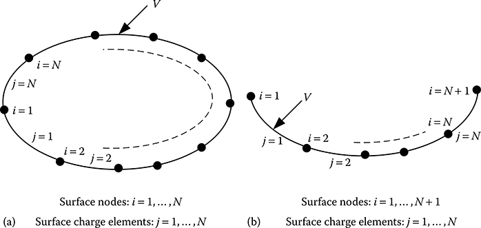
FIGURE 17.1
Surface charge elements and nodes on electrode boundary: (a) for closed-type boundary and (b) for open-type boundary.

Similar to CSM, SCSM also requires that at any one of these surface nodes, the potential resulting from superposition of effects all the surface charge elements is equal to the known electrode potential. The potential at any surface node due to a surface charge element is computed by integrating over the surface element considering a predetermined distribution of charge density along the surface element. Different types of charge density distribution may be considered. However, practical experience shows that linear charge density distribution gives accurate results for most of the practical cases. As a result, in this chapter, all subsequent discussions are based on linear distribution of charge density over a surface charge element. In SCSM, charge densities are considered at the surface nodes, the magnitudes of which are unknown and are to be solved. At any point on the jth surface charge element, the charge density σ(pelm) could be obtained from the charge densities of the nodes defining the surface element using linear charge density distribution. Then, at any surface node i, the potential due to the jth surface charge element will be given by

$ϕ_{i j} = \int_{e l m j} P_{i j} σ (pelm) d (pelm) (17.1)$

where:

P_ij is the potential coefficient which depends on the type of surface charge element
d(pelm) depends on the system configuration

For 2D or axi-symmetric systems, d(pelm) is length and the integration is carried out over a line element and for 3D configurations d(pelm) is area and the integration is carried out over an area element. Similar to CSM, potential coefficients are evaluated analytically for different types of surface charge elements by solving Laplace’s equation.

Electric field intensity components are obtained by differentiating Equation 17.1 as follows:

$E_{x, i j} = \int_{e l m j} - \frac{\partial P_{i j}}{\partial x} σ (pelm) d (pelm) (17.2a)$

$E_{y, i j} = \int_{e l m j} - \frac{\partial P_{i j}}{\partial y} σ (pelm) d (pelm) (17.2b)$

$E_{z, i j} = \int_{e l m j} - \frac{\partial P_{i j}}{\partial z} σ (pelm) d (pelm) (17.2c)$

When Equation 17.1 is applied at ith node for all the N number of surface charge elements, it gives the potential of node i, which according to Dirichlet’s condition should be equal to the known electrode potential, that is,

$ϕ_{i} = \sum_{j = 1}^{j = N} ϕ_{i j} = V (17.3)$

When Equation 17.3 is applied to N number of surface nodes, it leads to the following system of N linear equations for N unknown surface charge densities. In matrix form, it may be written as

$[\begin{matrix} ϕ_{11} ϕ_{12} \dots ϕ_{1 N} \\ ϕ_{21} ϕ_{22} \dots ϕ_{2 N} \\ ⋮ \\ ϕ_{N 1} ϕ_{N 2} \dots ϕ_{N N} \end{matrix}] = [V] (17.4)$

As in the case of CSM, in many cases, the effect of the ground plane is to be considered for electric field calculation. This plane can be taken into account by introducing the image of surface charge elements.

17.3 Surface Charge Elements in 2D and Axi-Symmetric Configurations

For the calculation of 2D and axi-symmetric fields, straight line and elliptical arc elements are most commonly used and are discussed here. A linear basis function is assumed for the description of charge density distribution along the element between the two nodes, which are the extremities of any given element.

In both the types of elements, as shown in Figure 17.2, a local coordinate ξ is introduced for the purpose of integration over the element, the value of which varies from −1 at node i to +1 at node i + 1.

17.3.1 Straight Line Element

With reference to Figure 17.2a, the location of any point lying on the element between node i and node i + 1 is given by

For 2D system:

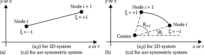
$\begin{matrix} x (ξ) = x_{i + 1} \frac{1 + ξ}{2} + x_{i} \frac{1 - ξ}{2} \\ y (ξ) = y_{i + 1} \frac{1 + ξ}{2} + y_{i} \frac{1 - ξ}{2} \end{matrix} (17.5)$

Images

FIGURE 17.2
Surface charge elements in 2D and axi-symmetric configurations: (a) straight line element and (b) elliptic arc element.

For axi-symmetric system:

$\begin{matrix} r (ξ) = r_{i + 1} \frac{1 + ξ}{2} + r_{i} \frac{1 - ξ}{2} \\ z (ξ) = z_{i + 1} \frac{1 + ξ}{2} + z_{i} \frac{1 - ξ}{2} \end{matrix} (17.6)$

The charge density at any point on the element between node i and node i + 1 is given by

$\begin{matrix} σ (ξ) = σ_{i + 1} \frac{1 + ξ}{2} + σ_{i} \frac{1 - ξ}{2} \end{matrix} (17.7)$

For 2D system, the field is independent of the direction normal to the plane of the paper and hence the charge at any point on the element is equivalent to an infinitely long line charge, extending up to infinity in a direction normal to the plane of the paper. As a result, for computing the potential coefficient, the expression for infinitely long line charge given by Equation 16.20 in Chapter 16 could be used in SCSM. Electric field intensity coefficients could be computed using the Equations 16.21 and 16.22 given in Chapter 16.

For an axi-symmetric system, the z-axis is the axis of symmetry and hence the charge at any point on the element is equivalent to a ring charge, when the element is not lying on the z-axis. As a result, for computing the potential coefficient, the expression for ring charge given by Equation 16.26 in Chapter 16 could be used in SCSM. Electric field intensity coefficients could be computed using Equations 16.27 and 16.28 given in Chapter 16. When the element lies on the z-axis, then the elemental charge length is equivalent to a finite length line charge. In such cases, for computing the potential coefficient, the expression for finite length line charge given by Equation 16.23 in Chapter 16 could be used in SCSM. Electric field intensity coefficients could be computed using Equations 16.24 and 16.25 given in Chapter 16.

Here, it is to be noted that the expressions given in Chapter 16 incorporates the effect of the image charge. Hence, if the image charge is not to be taken into account, then the part of the expression that represents the effect of image charge need not be taken into computation.

17.3.2 Elliptic Arc Element

For the description of the elliptic arc, parametric representation of an ellipse is commonly used. Angle θ is the parameter that varies linearly from node i and node i + 1 along the elliptic arc length.

With reference to Figure 17.2b, the parameter at any point on the element between node i and node i + 1 is given by

$\begin{matrix} θ (ξ) = θ_{i + 1} \frac{1 + ξ}{2} + θ_{i} \frac{1 - ξ}{2} \end{matrix} (17.8)$

and the location of any point lying on the element between node i and node i + 1 is given by

For 2D system:

$\begin{matrix} x (ξ) = x_{0} + A \cos θ (ξ) \\ y (ξ) = y_{0} + B sin θ (ξ) \end{matrix} (17.9)$

For axi-symmetric system:

$\begin{matrix} r (ξ) = r_{0} + A \cos θ (ξ) \\ z (ξ) = z_{0} + B sin θ (ξ) \end{matrix} (17.10)$

where:

(x₀,y₀) or (r₀,z₀) are the coordinates of the centre
A, B are the semi-major and semi-minor axes of the elliptic arc element, respectively

The charge density at any point on the elliptic arc element between node i and node i + 1 is also given by Equation 17.7. For both straight line and elliptic arc elements, the unit of charge density is Coulombs/m (C/m).

17.3.3 Contribution of Nodal Charge Densities to Coefficient Matrix

Consider four consecutive nodes defining three elements on any electrode boundary, as shown in Figure 17.3.

As per Equation 17.1, the potential of node M due to element M−1 is given by

$ϕ_{M, M - 1} = \int_{ξ = - 1}^{ξ = + 1} P_{M, M - 1} σ (ξ) d l (ξ) (17.11)$

Images

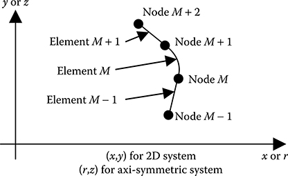
FIGURE 17.3
Pertaining to contribution of nodal charge densities to coefficient matrix.

where:

ξ = −1 at node M−1
ξ = +1 at node M for element M−1

Using Equation 17.7, Equation 17.11 can be modified as follows:

$\begin{matrix} ϕ_{M, M - 1} & = \int_{ξ = - 1}^{ξ = + 1} P_{M, M - 1} (σ_{M} \frac{1 + ξ}{2} + σ_{M - 1} \frac{1 - ξ}{2}) d l (ξ) \\ = σ_{M} \int_{ξ = - 1}^{ξ = + 1} P_{M, M - 1} \frac{1 + ξ}{2} d l (ξ) + σ_{M - 1} \int_{ξ = - 1}^{ξ = + 1} P_{M, M - 1} \frac{1 - ξ}{2} d l (ξ) \\ = σ_{M} C_{E M, M - 1} + o_{M - 1} C_{S M, M - 1} \end{matrix} (17.12)$

Similarly, the potential of node M due to element M will be given by

$\begin{matrix} ϕ_{M, M} & = \int_{ξ = - 1}^{ξ = + 1} P_{M, M} (σ_{M + 1} \frac{1 + ξ}{2} + σ_{M} \frac{1 - ξ}{2}) d l (ξ) \\ = σ_{M + 1} \int_{ξ = - 1}^{ξ = + 1} P_{M, M} \frac{1 + ξ}{2} d l (ξ) + σ_{M} \int_{ξ = - 1}^{ξ = + 1} P_{M, M} \frac{1 - ξ}{2} d l (ξ) \\ = σ_{M + 1} C_{E M, M} + σ_{M} C_{S M, M} \end{matrix} (17.13)$

Therefore, it may be seen that every nodal charge density will contribute twice towards the potential and also for electric field intensity of any node or point within the region of interest. This is because of the fact that every node belongs to two surface charge elements. In one element a given node will be the ending node, whereas in the next element, it will be the starting node. In Equations 17.12 and 17.13, the contribution of a nodal charge density is shown as C_S when it is the starting node of an element and as C_E when it is the ending node of another element. However, this is not valid for the starting node of the very first element and the ending node of the very last element of an open-type boundary, as shown in Figure 17.1b.

In light of Equations 17.12 and 17.13, the matrix of Equation 17.4 could be rewritten as follows for the closed-type boundary, as shown in Figure 17.1a.

$[\begin{matrix} (C_{S 1, 1} + C_{E 1, N}) (C_{S 1, 2} + C_{E 1, 1}) \dots (C_{S 1, i} + C_{E 1, i - 1}) \dots (C_{S 1, N} + C_{E 1, 1}) \\ (C_{S 2, 1} + C_{E 2, N}) (C_{S 2, 2} + C_{E 2, 1}) \dots (C_{S 2, i} + C_{E 2, i - 1}) \dots (C_{S 2, N} + C_{E 2, 1}) \\ ⋮ \\ (C_{S i, 1} + C_{E i, N}) (C_{S i, 2} + C_{E i, 1}) \dots (C_{S i, i} + C_{E i, i - 1}) \dots (C_{S i, N} + C_{E i, 1}) \\ ⋮ \\ (C_{S N, 1} + C_{E N, N}) (C_{S N, 2} + C_{E N, 1}) \dots (C_{S N, i} + C_{E N, i - 1}) \dots (C_{S N, N} + C_{E N, 1}) \end{matrix}] [\begin{matrix} σ_{1} \\ σ_{2} \\ ⋮ \\ σ_{i} \\ ⋮ \\ σ_{N} \end{matrix}] = [\begin{matrix} V \\ V \\ ⋮ \\ V \\ ⋮ \\ V \end{matrix}] (17.14)$

For open-type boundary, as shown in Figure 17.1b, Equation 17.14 will be modified as follows:

$[\begin{matrix} (C_{S 1, 1}) (C_{S 1, 2} + C_{E 1, 1}) \dots (C_{S 1, i} + C_{E 1, i - 1}) \dots (C_{E 1, N - 1}) \\ (C_{S 2, 1}) (C_{S 2, 2} + C_{E 2, 1}) \dots (C_{S 2, i} + C_{E 2, i - 1}) \dots (C_{E 2, N - 1}) \\ ⋮ \\ (C_{S i, 1}) (C_{S i, 2} + C_{E i, 1}) \dots (C_{S i, i} + C_{E i, i - 1}) \dots (C_{E i, N - 1}) \\ ⋮ \\ (C_{S N, 1}) (C_{S N, 2} + C_{E N, 1}) \dots (C_{S N, i} + C_{E N, i - 1}) \dots (C_{E N, N - 1}) \end{matrix}] [\begin{matrix} σ_{1} \\ σ_{2} \\ ⋮ \\ σ_{i} \\ ⋮ \\ σ_{N} \end{matrix}] = [\begin{matrix} V \\ V \\ ⋮ \\ V \\ ⋮ \\ V \end{matrix}] (17.15)$

The difference between the matrices of Equations 17.14 and 17.15 is that in Equation 17.15 the first and the last columns have only one term, either the starting or the ending term, in the matrix elements. This is due to the fact that for an open-type boundary the starting node of the very first element belongs to only one element as the starting node and the ending node of the very last element belongs also to only one element as the ending node. One more point to be noted is that for an open-type boundary, if there are N number of nodes, then there will be N − 1 number of elements instead of N. Accordingly the matrix elements of Equation 17.15 are different from those of Equation 17.14.

17.3.4 Method of Integration over a Surface Charge Element

In order to achieve good accuracy in SCSM, it is imperative that the integrations are carried out with high accuracy. It has been noted by the researchers that numerical integration by Gauss–Legendre Quadrature rule provides excellent accuracy. Hence, this integration rule is briefly discussed here.

Gauss–Legendre Quadrature rule approximates an integral as the sum of a finite number (n) of terms in the following way, by picking approximate values for n, w_i and ξ_i

$\int_{- 1}^{+ 1} f (ξ) d ξ ≅ \sum_{i = 1}^{n} w_{i} f (ξ_{i}) (17.16)$

where:

ξ_i is known as Gauss point or abscissa
The values of ξ_i are zeroes of the nth degree Legendre polynomial
w_i is the weight of the function value at ith Gauss point or abscissa

Although this rule is originally defined for the interval (−1,1), this is actually a universal function, because the limits of integration could be converted from any interval (a,b) to the Gauss–Legendre interval (−1,1) in the following manner

TABLE 17.1
High-Precision Abscissae and Weights of 16-Point Gauss–Legendre Quadrature Rule

Images

$\int_{a}^{b} f (ξ) d ξ ≅ \frac{b - a}{2} \sum_{i = 1}^{n} w_{i} f (\frac{b - a}{2} ξ_{i} + \frac{b + a}{2}) (17.17)$

In SCSM, 16-point or even 13-point Gauss–Legendre Quadrature rule gives excellent accuracy. Hence, abscissae and weights of 16-point Gauss–Legendre Quadrature rule are given in Table 17.1.

17.3.5 Electric Field Intensity Exactly on the Electrode Surface

It has already been discussed in Section 8.2.1 that the highest value of electric field intensity does not occur on the electrode surface, but occurs just off the electrode surface within the dielectric medium. Still it is relevant to compute the electric field intensity exactly on the surface. Here, it is to be noted that the electric field intensity is always directed along the normal to the surface at any point lying exactly on the electrode surface.

As in the case of electric potential given by Equation 17.12, the normal component of electric field intensity at node M due to element M−1 can be computed as follows:

$\begin{matrix} E_{N M, M - 1} & = \int_{ξ = - 1}^{ξ = + 1} F_{N M, M - 1} (σ_{M} \frac{1 + ξ}{2} + σ_{M - 1} \frac{1 - ξ}{2}) d l (ξ) \\ = σ_{M} \int_{ξ = - 1}^{ξ = + 1} F_{N M, M - 1} \frac{1 + ξ}{2} d l (ξ) + σ_{M - 1} \int_{ξ = - 1}^{ξ = + 1} F_{N M, M - 1} \frac{1 - ξ}{2} d l (ξ) \\ = σ_{M} A_{E M, M - 1} + σ_{M - 1} A_{S M, M - 1} \end{matrix} (17.18)$

where:

F_N is normal field intensity coefficient

Similarly, the normal component of electric field intensity at node M due to element M is given by

$\begin{matrix} E_{N M, M} & = \int_{ξ = - 1}^{ξ = + 1} F_{N M, M} (σ_{M + 1} \frac{1 + ξ}{2} + σ_{M} \frac{1 - ξ}{2}) d l (ξ) \\ = σ_{M + 1} \int_{ξ = - 1}^{ξ = + 1} F_{N M, M} \frac{1 + ξ}{2} d l (ξ) + σ_{M} \int_{ξ = - 1}^{ξ = + 1} F_{N M, M} \frac{1 - ξ}{2} d l (ξ) \\ = σ_{M + 1} A_{E M, M} + σ_{M} A_{S M, M} \end{matrix} (17.19)$

For any node i the normal component of electric field intensity due to all the elements on the electrode boundary could be obtained from Equations 17.14, 17.18 and 17.19 for closed-type boundary as follows:

$\begin{matrix} E_{N i} = (A_{S i, 1} + A_{E i, N}) σ_{1} + (A_{S i, 2} + A_{E i, 1}) σ_{2} + ...+ (A_{S i, i} + A_{E i, i - 1}) σ_{i} \\ +... + (A_{S i, N} + A_{E i, 1}) σ_{N} \end{matrix} (17.20)$

and from Equations 17.15, 17.18 and 17.19 for open-type boundary as follows:

$E_{N i} = A_{S i, 1} σ_{1} + (A_{S i, 2} + A_{E i, 1}) σ_{2} + ... + (A_{S i, i} + A_{E i, i - 1}) σ_{i} + ...+ A_{E i, N - 1} σ_{N} (17.21)$

Because node i has a charge density σ_i, there will be problem of singularity in evaluating the coefficient terms associated to σ_i. Therefore, the coefficients associated to σ_i are computed leaving aside a small part around node i. However, it may be mentioned here that in Gauss–Legendre Quadrature rule, the integrand is approximated at the selected abscissae, which do not coincide with the nodes lying at the extremities of the element. Hence, the integrand is not computed at the nodes and so singularity does not appear. But, to be precise and correct in computation, it is necessary to assume that the values obtained from Equations 17.20 and 17.21 are without the small part around the node under consideration. Then the charge on the small part left aside around node i is considered as a point charge of magnitude σ_i and the field intensity, which is normal to the electrode surface, due to this point charge is given by [(σ_i/2ε_rε₀)]. This additional normal electric field intensity has to be added to the value obtained either from Equation 17.20 or 17.21 to get the value exactly on the node.

17.4 SCSM Formulation for Multi-Dielectric Media

In the case of multi-dielectric configuration, free charges are present on the electrode boundaries and bound charges are present on the dielectric–dielectric boundaries, which appear due to dielectric polarization. In ideal condition, there should not be any free charge present on a dielectric–dielectric boundary. But in many practical cases, due to volume as well as surface conduction, partial discharge and so on, there could be free charges present on dielectric–dielectric boundary. In the case of Laplacian field, the free charge density on dielectric boundary is zero, while for Poissonian field the effect of the free charges present on the dielectric boundary needs to be taken into consideration.

In SCSM, Neumann condition for normal component of electric flux density is satisfied on dielectric–dielectric boundary as mentioned below:

$ε_{1} E_{n 1} - ε_{2} E_{n 2} = σ_{s} (17.22)$

where:

σ_s is free charge density on dielectric–dielectric boundary, which is finite for Poissonian field and is zero for Laplacian field

Consider a multi-electrode and multi-dielectric arrangement, as shown in Figure 17.4. For this arrangement, all the boundaries are discretized into suitable number of surface charge elements and the field at any point within the region of interest is due to the superimposed effect of all such surface charge elements.

Let there be ELB number of electrode boundaries and DLB number of dielectric–dielectric boundaries. At any node i on the dielectric boundary, the normal component of electric field intensity is computed as

Images

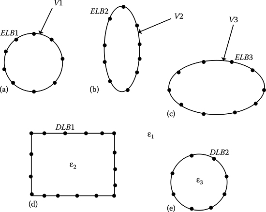
FIGURE 17.4
Schematic diagram of a multi-electrode and multi-dielectric arrangement. (a) ELB1, electrode boundary 1; (b) ELB2, electrode boundary 2; (c) ELB3, electrode boundary 3; (d) DLB1, dielectric boundary 1; (e) DLB2, dielectric boundary 2.

$E_{n, i}^{-} = \sum_{e = 1}^{E L B} E_{n, i} + \sum_{d = 1 (d \neq D L B i)}^{D L B} E_{n, i} + \sum_{d = (D L B i - A B)} E_{n, i} (17.23)$

where:

e and d denote electrode and dielectric boundaries, respectively
DLBi is the dielectric boundary on which the node i is located
AB is a small part around node i

The left-hand side of Equation 17.23 is denoted as $E_{n, i}^{-}$ , because the small part AB around node i is not considered for the computation. The terms on the right-hand side of Equation 17.23 are computed using either Equation 17.20 or 17.21.

Normal electric field intensity in free space due to the small part AB around node i can be written as follows, with orientation to side 1 of the dielectric–dielectric boundary:

$E_{1 n, i}^{A B} = - E_{2 n, i}^{A B} = \frac{σ_{i}}{2 ε_{0}} (17.24)$

Thus, the normal component of electric field intensity at the node i on both sides of the dielectric–dielectric boundary can be written as

$E_{1 n, i} = E_{n, i}^{-} + \frac{σ_{i}}{2 ε_{0}} = \sum_{e = 1}^{E L B} E_{n, i} + \sum_{d = 1 (d \neq D L B i)}^{D L B} E_{n, i} + \sum_{d = (D L B i - A B)} E_{n, i} + \frac{σ_{i}}{2 ε_{0}} (17.25)$

and

$E_{2 n, i} = E_{n, i}^{-} - \frac{σ_{i}}{2 ε_{0}} = \sum_{e = 1}^{E L B} E_{n, i} + \sum_{d = 1 (d \neq D L B i)}^{D L B} E_{n, i} + \sum_{d = (D L B i - A B)} E_{n, i} - \frac{σ_{i}}{2 ε_{0}} (17.26)$

Combining Equations 17.22, 17.25 and 17.26, the boundary condition can thus be written as

$\begin{matrix} ε_{1} (\sum_{e = 1}^{E L B} E_{n, i} + \sum_{d = 1 (d \neq D L B i)}^{D L B} E_{n, i} + \sum_{d = (D L B i - A B)} E_{n, i} + \frac{σ_{i}}{2 ε_{0}}) \\ - ε_{2} (\sum_{e = 1}^{E L B} E_{n, i} + \sum_{d = 1 (d \neq D L B i)}^{D L B} E_{n, i} + \sum_{d = (D L B i - A B)} E_{n, i} - \frac{σ_{i}}{2 ε_{0}}) = σ_{s, i} \end{matrix} (17.27)$

17.5 SCSM Formulation in 3D System

In contrast to finite element method (FEM), in SCSM only the boundary surfaces are approximated by finite number of boundary elements. The boundary elements are mainly of two types: (1) triangles and (2) rectangles. Depending on how precisely these boundary elements need to be defined, shape functions of different orders are used. In most of the practical cases, boundary elements are either of first order or of second order, which can be defined analytically by natural coordinate system. Thus, the problem of solving integral equations can be looked upon as defining a set of functions of equivalent surface charge densities defined on each boundary element.

Figure 17.5a and b show typical discretization of a multi-electrode multi-dielectric arrangement used in a gas-insulated system. The discretization is done by triangular elements. One of the main reasons for using triangular elements is that any irregular polygon can be looked upon as a union of several triangles. The simplicity of the approximating functions used with triangular elements lies in its two basic properties, namely, (1) these functions always ensure the continuity of the desired potential along all the boundaries between triangles provided only that continuity is imposed at the vertices of the triangle and (2) the approximations are independent of the global coordinates of the triangles.

Images

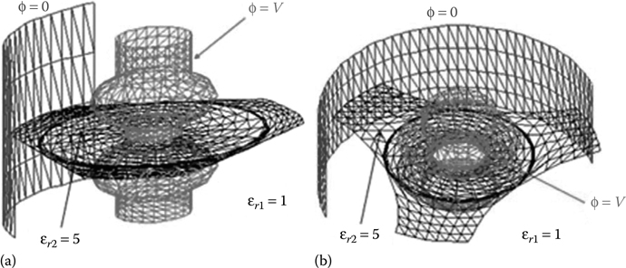
FIGURE 17.5
(See colour insert.) Discretization of a practical multi-electrode multi-dielectric arrangement using triangular elements: (a) view 1 and (b) view 2.

In order to obtain the numerical solution of integral equations, it is required to introduce basis functions of suitable order for approximating the surface charge density (σ) on each surface. Similar to the case of FEM, it is convenient to express the basis function in local coordinate system. In most of the cases, the boundary elements are approximated by first order polynomials, that is, using linear approximation. It follows that the number of nodes on each of the triangular boundary elements will be three. In other words, the surface charge densities are assumed at the vertices of each triangular boundary element. Thus, the surface charge density function over a boundary element can be written in terms of the shape functions as

$σ_{e l e} = L_{1} σ_{1} + L_{2} σ_{2} + L_{3} σ_{3} (17.28)$

where:

L₁ + L₂ + L₃ = 0

The shape functions and natural coordinates for linear triangular elements have been discussed in detail in Sections 15.4.4 and 15.4.5. Other types of surface elements have also been discussed in Section 15.4.6. The relationships described in the above-mentioned sections of Chapter 15 can be used here.

With reference to Figure 17.6, the contribution of a particular linear boundary element M to the potential at any arbitrary point G is given by

$ϕ_{G, M} = \frac{1}{4 π ε_{0}} \int_{0}^{11} \int_{0}^{- L 1} \frac{L_{1} σ_{1} + L_{2} σ_{2} + (1 - L_{1} - L_{2}) σ_{3}}{r_{G M} (L_{1}, L_{2})} | J (L_{1;} L_{2}) | d L_{1} d L_{2} (17.29)$

where:

J(L₁,L₂) is the Jacobian matrix of the transformation for shape functions

When expressed in natural (ξ − η) coordinates, Equation 17.29 is modified to

$ϕ_{G, M} = \frac{1}{4 π ε_{0}} \int_{0}^{11} \int_{0}^{- ξ} \frac{ξ σ_{1} + η σ_{2} + (1 - ξ - η) σ_{3}}{r_{G M} (ξ, η)} | J (ξ, η) | d ξ d η (17.30)$

where:

J(ξ,η) is the Jacobian matrix of the transformation for natural coordinates and is given in Section 15.4.5

Images

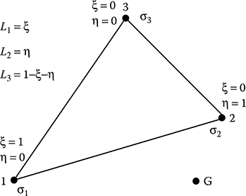
FIGURE 17.6
Linear triangular boundary element.

Equation 17.30 shows that potential coefficient has three terms as given below.

$\begin{matrix} P_{1} = \frac{1}{4 π ε_{0}} \int_{0}^{11} \int_{0}^{- ξ} \frac{ξ σ_{1}}{r_{G M} (ξ, η)} | J (ξ, η) | d ξ d η \\ P_{2} = \frac{1}{4 π ε_{0}} \int_{0}^{11} \int_{0}^{- ξ} \frac{η σ_{2}}{r_{G M} (ξ, η)} | J (ξ, η) | d ξ d η \\ P_{3} = \frac{1}{4 π ε_{0}} \int_{0}^{11} \int_{0}^{- ξ} \frac{(1 - ξ - η) σ_{3}}{r_{G M} (ξ, η)} | J (ξ, η) | d ξ d η \end{matrix} (17.31)$

Electric field intensity coefficients could be obtained in a similar manner.

17.6 Capacitive-Resistive Field Computation by SCSM

SCSM can be employed to compute capacitive-resistive field accurately in 2D, axi-symmetric and 3D systems including volume and surface resistances. The methodology for 2D and axi-symmetric systems are similar and are described in the next sub-section, whereas the 3D formulations are given in the subsequent sub-section.

17.6.1 Capacitive-Resistive Field Computation in 2D and Axi-Symmetric Systems

For capacitive-resistive field computation Dirichlet’s condition on the electrode boundary remains unaltered, but σ_s of Equation 17.22 need to be determined from the general condition of current density vector at node i to include volume and surface resistances in the following manner.

$J_{1 n, i} - J_{2 n, i} + Δ J_{s, i} + \frac{\partial σ_{s, i}}{\partial t} = 0 (17.32)$

With reference to Figure 15.11 of Chapter 15 and for isotropic media, Equation 17.32 can be rewritten as

$\frac{E_{1 n, i}}{ρ_{v 1}} - \frac{E_{2 n, i}}{ρ_{v 2}} + Δ J_{s, i} + \frac{\partial σ_{s, i}}{\partial t} = 0 (17.33)$

where:

ρ_vx is volume resistivity of dielectric x, x = 1,2

For sinusoidal fields, incorporating complex notations Equation 17.33 can be written as

$\frac{{\bar{E}}_{1 n, i}}{ρ_{v 1}} - \frac{{\bar{E}}_{2 n, i}}{ρ_{v 2}} + Δ {\bar{J}}_{s, i} + j ω {\bar{σ}}_{s, i} = 0 (17.34)$

With reference to Figure 15.13, surface current density term in Equation 17.34 can be written as

$Δ {\bar{J}}_{s, i} = \frac{1}{S (i)} [{\bar{ϕ}}_{i} (\frac{1}{R (i)} + \frac{1}{R (i + 1)}) - \frac{{\bar{ϕ}}_{i + 1}}{R (i + 1)} - \frac{{\bar{ϕ}}_{i - 1}}{R (i)}] (17.35)$

where:

R(i) and R(i + 1) are surface resistances corresponding to ith and (i + 1)th boundary node, respectively
S(i) is a small surface area corresponding to ith boundary node

The expressions for R(i) and S(i) are given for a 2D system in Equations 15.62 and 15.63, respectively, and for an axi-symmetric system in Equations 15.64 and 15.65, respectively, in Chapter 15.

Finally, Equations 17.27, 17.34 and 17.35 can be combined together in the following form.

$\frac{2 ({\bar{ε}}_{1} - {\bar{ε}}_{2})}{({\bar{ε}}_{1} + {\bar{ε}}_{2})} {\bar{E}}_{n, i} - \frac{2 j}{ω S (i) ({\bar{ε}}_{1} + {\bar{ε}}_{2})} [{\bar{ϕ}}_{i} (\frac{1}{R (i)} + \frac{1}{R (i + 1)}) - \frac{{\bar{ϕ}}_{i + 1}}{R (i + 1)} - \frac{{\bar{ϕ}}_{i - 1}}{R (i)}] + \frac{{\bar{σ}}_{i}}{2 ε_{0}} = 0 (17.36)$

where:

${\bar{ε}}_{x} = ε_{0} ε_{r x} - [j / (ω ρ_{υ x})]$ , x = 1,2 and ${\bar{E}}_{n, i}$ , are given in details in Equation 17.23 without complex notations

17.6.2 Capacitive-Resistive Field Computation in 3D System

Incorporating volume resistivity into a 3D capacitive-resistive field computation is similar to a 2D or an axi-symmetric system, because the current density due to volume resistance is caused by the normal component of the electric field intensity at a surface node, as given in Equation 17.33. Hence, volume resistivity could be incorporated by considering the permittivity of the dielectric medium as a complex quantity and expressing it as ${\bar{ε}}_{x} = ε_{0} ε_{r x} - [j / (ω ρ_{υ x})]$ , where, ε_x is the permittivity of medium x and ρ_vx is its volume resistivity.

However, incorporation of surface resistance into 3D capacitive-resistive field computation requires special treatment as discussed below. In this treatment, hexagonal discretization using triangular elements has been considered. As shown in Figure 17.7, the target node 0 is connected to six other nodes, namely, 1, 2, 3, 4, 5 and 6. The potentials of these nodes are V₀, V₁, V₂, V₃, V₄, V₅ and V₆, respectively, as shown in Figure 17.7. R₁, R₂, R₃, R₄, R₅ and R₆ are the resistances of the branches 01, 02, 03, 04, 05 and 06, respectively. Surface currents flowing through the branches 01, 02, 03, 04, 05 and 06 are I₁, I₂, I₃, I₄, I₅ and I₆, respectively. The directions of all these currents are assumed to be from node 0 to node k, k = 1, 6.

Images

FIGURE 17.7
Incorporation of surface resistance into SCSM 3D formulation.

Then, application of Kirchhoff’s current law at node 0 gives

$\sum_{i = 1}^{6} \frac{V_{0} - V_{i}}{R_{i}} = 0 (17.37)$

For AC field, charge could be computed in the following way.

$q_{s} (t) = \int i_{s} (t) d t = \int I_{s m} e^{j ω t} d t = \frac{i_{s} (t)}{j ω} (17.38)$

Removing t and bringing in complex notation and combining Equations 17.37 and 17.38, surface charge can be written as

$\bar{q_{s}} = \frac{1}{j ω} \sum_{i = 1}^{6} \frac{{\bar{V}}_{0} - {\bar{V}}_{i}}{R_{i}} (17.39)$

Then, the surface charge density around node 0 over the surface can be obtained as follows:

$\bar{σ_{s}} = \frac{1}{j ω S_{0}} \sum_{i = 1}^{6} \frac{{\bar{V}}_{0} - {\bar{V}}_{i}}{R_{i}} (17.40)$

where:

S₀ is a surface area around the node 0

As depicted in Figure 17.7, A, B, C, D, E and F are the mid points of 01, 02, 03, 04, 05 and 06, respectively. S₀ is the summation of the areas of the triangles 0AB, 0BC, 0CD, 0DE, 0EF and 0FA such that

$S_{0} = \frac{1}{4} (Δ_{0 A B} + Δ_{0 B C} + Δ_{0 C D} + Δ_{0 D E} + Δ_{0 E F} + Δ_{0 F A}) (17.41)$

where:

Δ is the area of the triangle denoted by the suffix

Surface resistance between two nodes is obtained in the following way. Figure 17.8 shows two adjacent triangular elements 056 and 061 of Figure 17.7. Consider that the surface resistance R₆ between the nodes 0 and 6 is to be computed, between which surface current I₆ is flowing, as shown in Figure 17.7. Now the side 06 belongs to both the triangular elements 056 and 061. As shown in Figure 17.8, OG and OH are the medians of triangular elements 056 and 061, respectively. Thus,

$Δ_{0 G 6} = \frac{1}{2} Δ_{056} and Δ_{06 H} = \frac{1}{2} Δ_{061} (17.42)$

Let the length of 06 be L₀₆ and the equivalent lengths that are normal to the direction of flow of I₆ are as shown by the hatched lines in the triangles 0G6 and 06H in Figure 17.8. Let the height of the triangles 0G6 and 06H be L_h1 and L_h2, respectively. Considering L₀₆ as the base of the triangles 0G6 and 06H, L_h1 and L_h2 can be obtained as

Images

FIGURE 17.8
Computation of surface resistance on the boundary.

$Δ_{0 G 6} = \frac{1}{2} L_{h 1} L_{06} and Δ_{06 H} = \frac{1}{2} L_{h 2} L_{06} (17.43)$

Combining Equations 17.42 and 17.43,

$L_{h 1} = 2 \frac{Δ_{0 G 6}}{L_{06}} = \frac{Δ_{056}}{L_{06}} and L_{h 2} = 2 \frac{Δ_{06 H}}{L_{06}} = \frac{Δ_{061}}{L_{06}} (17.44)$

Because the surface resistance associated to the side 06 is R₆,

$R_{6} = (ρ_{s, 06} \frac{L_{06}}{L_{h 1}}) ‖ (ρ_{s, 06} \frac{L_{06}}{L_{h 2}}) = ρ_{s, 06} \frac{L_{06}}{L_{h 1} + L_{h 2}} (17.45)$

Combining Equations 17.44 and 17.45

$R_{6} = ρ_{s, 06} \frac{L_{06}^{2}}{Δ_{056} + Δ_{061}} (17.46)$

where:

ρ_s,06 is the surface resistivity associated to side 06

In the same way, the surface resistance associated to all the sides, as shown in Figure 17.7 can be written as follows:

$\begin{matrix} R_{1} = ρ_{s, 01} \frac{L_{01}^{2}}{Δ_{061} + Δ_{012}}, R_{2} = ρ_{s, 02} \frac{L_{02}^{2}}{Δ_{012} + Δ_{023}}, R_{3} = ρ_{s, 03} \frac{L_{03}^{2}}{Δ_{023} + Δ_{034}} \\ R_{4} = ρ_{s, 04} \frac{L_{04}^{2}}{Δ_{034} + Δ_{045}} and R_{5} = ρ_{s, 05} \frac{L_{05}^{2}}{Δ_{045} + Δ_{056}} \end{matrix} (17.47)$

From Equations 17.46 and 17.47 it is obvious that only half the area of the triangles to which the resistance path belongs should be considered while approximating the equivalent length perpendicular to the current path. Otherwise, every triangular element would have been considered twice while computing the resistance of the adjacent sides.

Then the Neumann condition at node 0 on dielectric–dielectric boundary is satisfied as follows:

$ε_{1} {\bar{E}}_{n 1, 0} - ε_{2} {\bar{E}}_{n 2, 0} = {\bar{σ}}_{s, 0} (17.48)$

where:

${\bar{σ}}_{s, 0}$ is obtained from Equation 17.40 and is given below in expanded form

${\bar{σ}}_{s, 0} = \frac{1}{j ω S_{0}} [\begin{matrix} {\bar{V}}_{0} (\frac{1}{R_{1}} + \frac{1}{R_{2}} + \frac{1}{R_{3}} + \frac{1}{R_{4}} + \frac{1}{R_{5}} + \frac{1}{R_{6}}) \\ - (\frac{{\bar{V}}_{1}}{R_{1}} + \frac{{\bar{V}}_{2}}{R_{2}} + \frac{{\bar{V}}_{3}}{R_{3}} + \frac{{\bar{V}}_{4}}{R_{4}} + \frac{{\bar{V}}_{5}}{R_{5}} + \frac{{\bar{V}}_{6}}{R_{6}}) \end{matrix}] (17.49)$

where:

${\bar{V}}_{k}$ is the potential of the kth node
R_k is the resistance of the side connecting node 0 and the kth node. R_k is given by Equation 17.46 or 17.47
S₀ is the area associated with node 0 as given by Equation 17.41

In order to compute capacitive-resistive fields incorporating both volume and surface resistances, Equation 17.48 is modified by bringing in complex permittivity.

${\bar{ε}}_{1} {\bar{E}}_{n 1, 0} - {\bar{ε}}_{2} {\bar{E}}_{n 2, 0} = {\bar{σ}}_{s, 0} (17.50)$

where:

${\bar{ε}}_{x} = ε_{0} ε_{r x} - [j / (ω ρ_{υ x})]$ , x = 1,2 and ρ_vx is volume resistivity of medium x
${\bar{σ}}_{s, 0}$ , is computed according to Equation 17.49

17.7 SCSM Examples

17.7.1 Cylinder Supported on Wedge

In many practical cases, electrodes are supported by insulating wedges. Figure 17.9 shows a metallic cylindrical electrode supported by solid insulating wedge. The point where the electrode touches the solid insulating material is called triple junction, as electrode, solid insulating material and gaseous dielectric (air in this case) meet at this point. The dimension of air gap between the electrode and the solid insulation depends on the angle α. Ideally the angle α should be made 90°. But it is not always possible to make it so. Hence, it is important to study the effect of the angle α on the field distribution particularly around the triple junction, where field concentration takes place. In this example, the metallic electrode boundary and the solid–air dielectric interfaces on both the sides of the electrode are discretized by line and arc elements as this is a 2D case study. The elements are located between two successive nodes as marked on Figure 17.9. The sizes of the elements need to be adjusted according to the field concentration. The element lengths are small near the triple junction while such lengths could be higher on those sections of the solid–air dielectric interface which are away from the electrode or triple junction. The effect of the earth surface is taken into account by considering images of surface charge elements.

Images

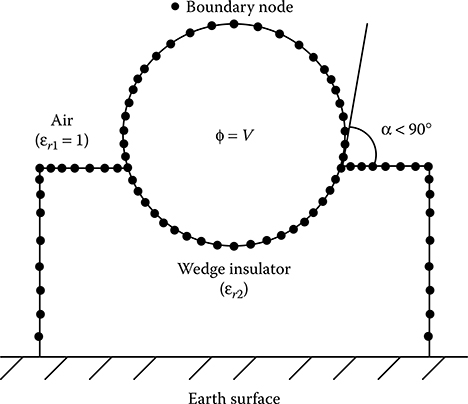
FIGURE 17.9
SCSM simulation of cylindrical electrode supported by solid insulating wedge.

17.7.2 Conical Insulator in Gas-Insulated System

Conical spacers are used in gas insulated substation (GIS) for providing insulating support to the live central conductor. The shape of the conductor at the junction of the electrode and solid spacer at both live and earth ends are suitably designed to reduce field concentration at these critical locations. Consequently, such electrode spacer configuration needs to be analyzed carefully from electrical field distribution viewpoint as the dimensions of GIS are relatively small and hence the margin of error is also small. Figure 17.10 shows a typical conical spacer with central and outer conductor arrangement used in GIS. It is an axi-symmetric configuration and is simulated by line and arc elements lying between two successive nodes as marked on Figure 17.10. There are four boundaries in this case that need to be discretized by boundary elements, for example, live conductor boundary, earthed conductor boundary and two solid insulation-SF₆ gas interfaces. The element lengths are to be adjusted according to the nature of field distribution. The elements near the spacer are smaller in size, while the elements on the sections of the electrodes away from the spacer are relatively larger. To avoid any edge effect affecting the results near the spacer, the electrode boundaries at the top and bottom of Figure 17.10 are to be considered extended up to a considerable distance from the spacer. But for simplicity it is not shown in Figure 17.10. In high-voltage DC (HVDC) GIS, conical spacers are often coated with a lossy dielectric for reducing problems due to charge accumulation. Such cases could also be studied by considering suitable surface resistivity along the two surfaces of the spacer.

Images

FIGURE 17.10
SCSM simulation of conical insulator used in GIS.

17.7.3 Metal Oxide Surge Arrester

Images

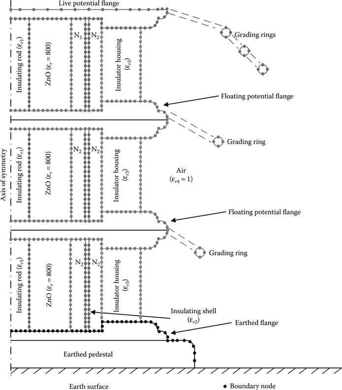
FIGURE 17.11
(See colour insert.) SCSM simulation of multiple unit assembly of metal oxide surge arrester.

For high-voltage–high-energy cases, the assembly of multiple units of metal oxide surge arresters are commonly used in power system. As shown in Figure 17.11, the metal oxide elements are held together by a central insulating rod and are placed within an insulating shell. Then this arrangement is housed in a protective outer cover very often made of porcelain. Nowadays, polymeric insulation is also used for outer covering. To provide an inert atmosphere within the insulator housing, N₂ gas is put instead of air. To linearize field distribution as much as possible field grading rings are used at the top live flange in all the applications. Sometimes grading rings are also used at the intermediate connecting flanges, as shown in Figure 17.11. The intermediate metallic flanges and the associated grading rings are floating potential electrodes and need to be simulated accordingly. The grading rings are closed-type boundaries while the other boundaries are open-type boundaries in this axi-symmetric example. The metal oxide elements have a dielectric constant of around 800 and very high resistivity before the start of conduction. The following are conductor boundaries that need to be simulated by boundary elements: (1) live flange boundary; (2) earthed flange boundary; (3) intermediate flange boundaries (two numbers), which are floating potential boundaries; (4) live potential grading rings (three numbers) and (5) floating potential grading rings (two numbers). There are several dielectric–dielectric boundaries in this example that are also to be simulated by boundary elements: (1) insulating rod–metal oxide boundary; (2) metal oxide–N₂ boundary; (3) N₂–insulating shell boundaries (two numbers); (4) N₂–insulator housing boundary and (5) insulator housing–air boundary. Line and arc elements are used for simulation. Change of resistance of metal oxide elements could be incorporated in field computation by considering appropriate value of volume resistivity of metal oxide elements.

17.7.4 Condenser Bushing of Transformer

Condenser bushings are very often used in high-voltage transformers (Figure 17.12). In this type of bushings floating potential grading electrodes are embedded in solid insulation (typically paper) to get a better field distribution. Consequently, it is practically important to study the electric field distribution in such bushing configuration. It is an axi-symmetric case with multiple electrode as well as dielectric boundaries. There are three types of electrode boundaries: (1) live central conductor boundary, (2) earthed metallic tank boundary and (3) floating potential grading electrode boundaries. It is to be noted here that these grading electrodes are very thin in dimension and SCSM is particularly useful in simulating such thin electrodes. There are following dielectric–dielectric boundaries, which are to be simulated by boundary elements: (1) paper–transformer oil boundary; (2) paper–porcelain boundary and (3) porcelain–air boundary. When the paper becomes aged with service, then conduction through paper insulation increases, which can be incorporated in field computation by assuming a suitable value of volume resistivity of paper insulation. Similarly, the volume conduction in transformer oil could also be duly considered in field computation by choosing the required value of volume resistivity of transformer oil. The surface pollution of porcelain outer cover could be taken into account by considering appropriate value of surface resistivity along porcelain–air boundary.

Images

FIGURE 17.12
SCSM simulation of condenser bushing used in high-voltage transformers.

Objective Type Questions

1. Indirect boundary element method is also known as

a. Charge simulation method

b. Volume charge simulation method

c. Surface charge simulation method

d. Region-oriented charge simulation method

2. In surface charge simulation method, which of the following functions are taken as unknown functions along the discrete boundary elements?

a. Surface charge density

b. Electric potential

c. Electric field intensity

d. Both (b) and (c)

3. In surface charge simulation method, Fredholm’s integral equations are used, in which

a. The kernel function is the potential and field coefficients and the weight function is the charge

b. The kernel function is the potential and field coefficients and the weight function is the charge density

c. The kernel function is the charge density and the weight function is the potential and field coefficients

d. The kernel function is the charge and the weight function is the potential and field coefficients

4. In surface charge simulation method, which of the following are discretized?

a. Entire volume of the regions of interest

b. All the boundaries of the regions of interest

c. Only the electrode boundaries

d. Only the dielectric–dielectric boundaries

5. If σ(i) is the equivalent surface charge density at any point i on the boundary, then the electric field intensity due to a small area around that point is given by

a. σ_iε₀

b. σ_i/ε₀

c. σ_i2ε₀

d. σ_i/(2ε₀)

6. For the calculation of 2D and axi-symmetric fields using surface charge simulation method, most commonly used elements are

a. Straight line and triangular elements

b. Elliptic arc and triangular elements

c. Straight line and elliptic arc elements

d. Straight line and circular arc elements

7. For the calculation of 3D fields using surface charge simulation method, most commonly used element is

a. Curvilinear triangle

b. Curvilinear rectangle

c. Curvilinear square

d. Irregular polygon

8. In surface charge simulation method, for an open-type boundary if the number of surface charge elements is N, then the number of surface nodes is

a. N − 2

b. N − 1

c. N

d. N + 1

9. In surface charge simulation method, for a closed-type boundary if the number of surface charge elements is N, then the number of surface nodes is

a. N − 2

b. N − 1

c. N

d. N + 1

10. In surface charge simulation method, for the computation of electric potential in a 2D or an axi-symmetric system, the integration is carried out over a

a. Line

b. Triangle

c. Quadrilateral

d. Volume

11. For a 2D field computation by surface charge simulation method, which one of the following charge configurations could be used?

a. Point charge

b. Infinite length line charge

c. Finite length line charge

d. Ring charge

12. For an axi-symmetric field computation by surface charge simulation method, which one of the following charge configurations could be used?

a. Point charge

b. Finite length line charge

c. Ring charge

d. All of the above

13. For 2D and axi-symmetric field computation by surface charge simulation method using linear basis function, charge density of unknown magnitude is considered on the discrete boundary elements

a. At the mid-point of the element

b. At the extremities of the element

c. Near but not at the mid-point of the element

d. Near but not at the extremities of the element

14. In surface charge simulation method, which one of the following integration rules gives excellent accuracy?

a. Trapezoidal rule

b. Simpson’s rule

c. Romberg’s rule

d. Gauss–Legendre Quadrature rule

15. In surface charge simulation method, the simplicity of the approximating functions used with triangular elements lies in which of the following basic properties

a. These functions always ensure the continuity of the desired potential along all the boundaries between triangles provided only that continuity is imposed at the vertices of the triangle

b. The approximations are independent of the global coordinates of the triangles

c. The approximations are independent of the local coordinates of the triangles

d. Both (a) and (b)

16. Surface charge simulation method formulations give rise to a coefficient matrix that by property is a

a. Sparse matrix

b. Nearly full matrix

c. Diagonal matrix

d. Unit matrix

17. At any node i on the dielectric boundary, let the normal component of electric field intensity be $E_{n, i}^{-}$ , when the small area AB around node i is not considered in the computation. Then which one of the following is incorporated to compute the normal component of electric field intensity at node i

a. σ_i/(2ε₀)

b. σ_i 2ε₀

c. σ_i/ε₀

d. σ_iε₀

18. The basic formulations of surface charge simulation method for capacitive field can be used for capacitive-resistive field, when

a. Only real quantities are used

b. Complex potentials are used

c. Complex charge densities are used

d. Both (b) and (c)

19. In surface charge simulation method, volume resistivity could be incorporated by expressing the permittivity of the dielectric medium as

a. ${\bar{ε}}_{x} = ω ρ_{υ x} - [j / (ε_{0} ε_{r x})]$

b. ${\bar{ε}}_{x} = ω ρ_{υ x} - j ε_{0} ε_{r x}$

c. ${\bar{ε}}_{x} = ε_{0} ε_{r x} - [j / (ω ρ_{υ x})]$

d. ${\bar{ε}}_{x} = ε_{0} ε_{r x} - j ω ρ_{υ x}$

20. By considering the general condition of current density vector at any node which one of the following could be included in field computation by surface charge simulation method?

a. Volume resistance

b. Surface resistance

c. Both (a) and (b)

d. Space charges

Answers:

1) c;

2) a;

3) b;

4) b;

5) d;

6) c;

7) a;

8) d;

9) c;

10) a;

11) b;

12) d;

13) b;

14) d;

15) d;

16) b;

17) a;

18) d;

19) c;

20) c

Bibliography

1. S. Sato and W.S. Zaengl, ‘Effective 3-dimensional electric field calculation by surface charge simulation method’, IEEE Proceedings A, Vol. 133, No. 2, pp. 77–83, 1986.

2. T. Kouno, ‘Computer calculation of electric fields’, IEEE Transactions on Electrical Insulation, Vol. 21, No. 6, pp. 869–872, 1986.

3. H. Tsuboi and T. Misaki, ‘The optimum design of electrode and insulator contours by nonlinear programming using the surface charge simulation method’, IEEE Transactions on Magnetics, Vol. 24, No. 1, pp. 35–38, 1988.

4. B.L. Qin, G.Z. Chen, Q. Qiao and J.N. Sheng, ‘Efficient computation of electric field in high voltage equipment’, IEEE Transactions on Magnetics, Vol. 26, No. 2, pp. 387–390, 1990.

5. H. Steinbigler, D. Haller and A. Wolf, ‘Comparative analysis of methods for computing 2-D and 3-D electric fields’, IEEE Transactions on Electrical Insulation, Vol. 26, No. 3, pp. 529–536, 1991.

6. D. Beatovic, P.L. Levin, S. Sadovic and R. Hutnak, ‘A Galerkin formulation of the boundary element for two-dimensional and axi-symmetric problems in electrostatics’, IEEE Transactions on Electrical Insulation, Vol. 27, No. 1, pp. 135–143, 1992.

7. Z. Andjelic, B. Krstajic, S. Milojkovic, A. Blaszczyk, H. Steinbigler and M. Wohlmuth, Integral Methods for the Calculation of Electric Fields, Scientific Series of the International Bureau, Vol. 10, Forschungszentrum Jülich GmbH, Germany, 1992.

8. J. Zhou, G.D. Theophilus and K.D. Srivastava, ‘Pre-breakdown field calculations for charged spacers in compressed gases under impulse voltages’, Proceedings of the IEEE ISEI, Baltimore, MD, pp. 273–278, July 3–8, IEEE Publication, 1992.

9. P.L. Levin, A.J. Hansen, D. Beatovic, H. Gan and J.H. Petrangelo, ‘A unified boundary-element finite-element package’, IEEE Transactions on Electrical Insulation, Vol. 28, No. 2, pp. 161–167, 1993.

10. F. Gutfleisch, H. Singer, K. Foerger and J.A. Gomollon, ‘Calculation of HV fields by means of the boundary element method’, IEEE Transactions on Power Delivery, Vol. 9, No. 2, pp. 743–749, 1994.

11. G. Mader and F.H. Uhlmann, ‘Computation of 3-D capacitances of transmission line discontinuities with the boundary element method’, Second International Conference on Computation in Electromagnetics, London, pp. 8–11, April 12–14, IEE (UK) Publication, 1994.

12. J. Weifang, W. Huiming and E. Kuffel, ‘Application of the modified surface charge simulation method for solving axial symmetric electrostatic problems with floating electrodes’, Proceedings of the IEEE ICPADM, Brisbane, Australia, Vol. 1, pp. 28–30, July 3–8, IEEE Publication, 1994.

13. A. Vishnevsky and A. Lapovok, ‘Conservative methods in boundary-element calculations of static fields’, IEEE Proceedings – Science, Measurement and Technology, Vol. 142, No. 2, pp. 151–156, 1995.

14. R. Schneider, P.L. Levin and M. Spasojevic, ‘Multiscale compression of BEM equations for electrostatic systems’, IEEE Transactions on Dielectrics & Electrical Insulation, Vol. 3, No. 4, pp. 482–493, 1996.

15. E. Cardelli and L. Faina, ‘Open-boundary, single-dielectric charge simulation method with the use of surface simulating charges’, IEEE Transactions on Magnetics, Vol. 33, No. 2, pp. 1192–1195, 1997.

16. S. Chakravorti and H. Steinbigler, ‘Electric field calculation including surface and volume resistivities by boundary element method’, Journal of the Institution of Engineers (India): Electrical Engineering Division, Vol. 78, No. 1, pp. 17–23, 1997.

17. N. de Kock, M. Mendik, Z. Andjelic and A. Blaszczyk, ‘Application of the 3D boundary element method in the design of EHV GIS components’, IEEE Electrical Insulation Magazine, Vol. 14, No. 3, pp. 17–22, 1998.

18. S. Chakravorti and H. Steinbigler, ‘Capacitive-resistive field calculation in and around HV bushings by boundary element method’, IEEE Transactions on Dielectrics & Electrical Insulation, Vol. 5, No. 2, pp. 237–244, 1998.

19. A. Ahmed, H. Singer and P.K. Mukherjee, ‘A numerical model using surface charges for the calculation of electric fields and leakage currents on polluted insulator surfaces’, Proceedings of the IEEE CEIDP, Atlanta, GA, Vol. 1, pp. 116–119, April 30–May 3, IEEE Publication, 1998.

20. B.Y. Lee, S.H. Myung, J.K. Park, S.W. Min and E.S. Kim, ‘The use of rational B-spline surface to improve the shape control for three-dimensional insulation design and its application to design of shield ring’, IEEE Transactions on Power Delivery, Vol. 13, No. 3, pp. 962–968, 1998.

21. P.K. Mukherjee, A. Ahmed and H. Singer, ‘Electric field distortion caused by asymmetric pollution on insulator surfaces’, IEEE Transactions on Dielectrics & Electrical Insulation, Vol. 6, No. 2, pp. 175–180, 1999.

22. A. Ahmed and H. Singer, ‘New modelling of the boundary between wet and dry zones on the surface of polluted high-voltage insulators’, Proceedings of the 11th ISH Symposium, London, Vol. 2, pp. 35–38, 1999.

23. S. Chakravorti and H. Steinbigler, ‘Boundary element studies on insulator shape and electric field around HV insulators with or without pollution’, IEEE Transactions on Dielectrics & Electrical Insulation, Vol. 7, No. 2, pp. 169–176, 2000.

24. A. Ahmed and H. Singer, ‘Effect of thermal capacities of ceramic insulators on their electrical and thermal analysis under contaminated surface conditions’, Proceedings of the IEEE CEIDP, Victoria, BC, Canada, Vol. 1, pp. 238–241, October 15–18, IEEE Publication, 2000.

25. S. Hamada and T. Takuma, ‘Electrostatic field calculation of multi-particle systems with and without contact points by the surface charge simulation method’, Proceedings of the 7th IEEE ICPADM, Nagoya, Japan, Vol. 1, pp. 27–32, June 1–4, IEEE Publication, 2003.

26. J.A. Gomollon and R. Palau, ‘Steady state 3-D-field calculations in three-phase systems with surface charge method’, IEEE Transactions on Power Delivery, Vol. 20, No. 2, pp. 919–924, 2005.

27. B. Zhang, S. Han, J. He, R. Zeng and P. Zhu, ‘Numerical analysis of electric-field distribution around composite insulator and head of transmission tower’, IEEE Transactions on Power Delivery, Vol. 21, No. 2, pp. 959–965, 2006.

28. B. Zhang, J. He, X. Cui, S. Han and J. Zou, ‘Electric field calculation for HV insulators on the head of transmission tower by coupling CSM with BEM’, IEEE Transactions on Magnetics, Vol. 42, No. 4, pp. 543–546, 2006.

29. W. Ling, Z. Rong, B. Zhang, G. Shanqiang, C. Lian and H. Jinliang, ‘Electric-field calculation for hot-line working on the head of transmission tower’, 12th Biennial IEEE Conference on Electromagnetic Field Computation, Miami, FL, p. 194, April 30–May 3, IEEE Publication, 2006.

30. B. Zhang, J. Zhao, R. Zeng and J. He, ‘Numerical analysis of DC current distribution in AC power system near HVDC system’, IEEE Transactions on Power Delivery, Vol. 23, No. 2, pp. 960–965, 2008.

31. S. Hamada and T. Kobayashi, ‘Analysis of electric field induced by ELF magnetic field utilizing fast-multipole surface-charge simulation method for voxel data’, Electrical Engineering in Japan, Vol. 165, No. 4, pp. 1–10, 2008.

32. S. Hamada, M. Kitano and T. Kobayashi, ‘Accuracy estimation of induced electric field calculated by fast-multipole surface-charge-simulation method for voxel data’, IEEE Transactions on Fundamentals and Materials, Vol. 128, No. 4, pp. 223–234, 2008.

33. C. Zhuang, R. Zeng, B. Zhang, P. Zhu, L. Wang and J. He, ‘The optimization of entering route for live working on 750 kV transmission towers by space electric-field analysis’, IEEE Transactions on Power Delivery, Vol. 25, No. 2, pp. 987–994, 2010.

34. J.A. Gomollon, E. Santome and R. Palau, ‘Calculation of 3D-capacitances with surface charge method by means of the basis set of solutions’, IEEE Transactions on Dielectrics & Electrical Insulation, Vol. 17, No. 1, pp. 240–246, 2010.

35. B.S. Reddy and U. Kumar, ‘Simulation of potential and electric field profiles for transmission line insulators’, International Journal of Modelling and Simulation, Vol. 30, No. 4, pp. 490–498, 2010.

36. B.S. Reddy and U. Kumar, ‘Investigations on the corona performance of a ceramic disc insulators integrated with field reduction electrode’, IEEE Industry Applications Society Annual Meeting, Houston, TX, pp. 1–8, October 3–7, IEEE Publication, 2010.

37. L. Xiaoming, W. Qi, C. Yundong and X. Qiumin, ‘Analyses of electric field for vacuum circuit breaker using response surface-charge simulation method’, Proceedings of the Asia-Pacific Power and Energy Engineering Conference, Chengdu, China, pp. 1–4, March 28–31, IEEE Publication, 2010.

38. S.S. Chowdhury, A. Lahiri and S. Chakravorti, ‘Surface resistance modified electric field computation in asymmetric configuration using surface charge simulation method: A new approach’, IEEE Transactions on Dielectrics & Electrical Insulation, Vol. 19, No. 3, pp. 1068–1075, 2012.

..................Content has been hidden....................

You can't read the all page of ebook, please click here login for view all page.

Table of Contents for 17. Numerical Computation of High-Voltage Field by Surface Charge Simulation Method

Create new playlist

Sign In

Sign Up

Answers:

Table of Contents for
17. Numerical Computation of High-Voltage Field by Surface Charge Simulation Method