11. Conformal Mapping

Search in book...
Toggle Font Controls
Create new playlist

Name your new playlist

Playlist description (optional)
Sign In

Email address

Password

Forgot Password?

or

Continue with Facebook

Continue with Google
Sign Up

Full Name

Email address

Confirm Email Address

Password

or

Continue with Facebook

Continue with Google

ABSTRACT Conformal mapping is a useful technique in the area of complex analysis and has many applications in different practical configurations. There are several problems in engineering that can be expressed in terms of functions of a complex variable, which involve complicated geometries. In such cases, by choosing an appropriate mapping function, the problem having inconvenient geometry can be transformed into a problem having much more convenient geometry. Conformal mapping is a technique that allows one to take hard problems, map them onto a coordinate system, where they are convenient to solve, find the solution and then map the solution back to the original system. This chapter gives a brief discussion on conformal mapping and some of its applications in solving practical problems in electrostatics.

11.1 Introduction

Analytical solutions to many field problems, particularly Dirichlet problems, can be obtained using methods such as Fourier series and integral transforms. These methods are applicable only for simple regions and the solutions are either infinite series or improper integrals, which are difficult to evaluate. Closed-form solutions to many Dirichlet problems can be obtained using conformal mapping, which is a similarity transformation. If a function is harmonic, that is, it satisfies Laplace’s equation ${\vec{\nabla}}^{2} f = 0$ , then the transformation of such a function via conformal mapping is also harmonic. Hence, equations in relation to any field that can be represented by a potential function can be solved with the help of conformal mapping. However, conformal mapping can only be employed in two-dimensional fields. If the solution for potential field is required in three-dimensional cases, then conformal mapping is applicable to only those configurations where the potential field is translationally invariant along any one of the three axes. The two-dimensional potential fields that can be solved by conformal mapping are static electric fields, static magnetic fields, static electric flow fields, stationary thermal flow fields, stationary hydrodynamic flow fields to name a few. According to Riemann mapping theorem any two regions with same connectivity may be conformally mapped to one another. But in practical applications, conformal mapping is used only in those cases where the maps take simpler, explicit forms, so that one may carry out actual calculations with those maps.

As the application of conformal mapping is limited to variables, which solve the Laplace’s equation for two-dimensional fields, one such variable of practical interest is the electrostatic potential in a region of space that is free of charges. This chapter, therefore, focuses on application of conformal mapping to determine electrostatic potential field by solving two-dimensional Laplace’s equation.

11.2 Basic Theory of Conformal Mapping

Conformal transformation is based on the properties of analytic functions. Let z = x + iy be a complex variable such that the real and imaginary parts x and y are real-valued variables, and f(z) = u(z) + i v(z) = u(x,y) + i v(x,y) be a complex-valued function such that the real and imaginary parts u and v are real- and single-valued functions of real-valued variables x and y.

If the derivative of f(z) exists at a point z, then the partial derivatives of u and v exist at that point and obey the Cauchy–Riemann equations as follows.

$\frac{\partial u}{\partial x} = \frac{\partial v}{\partial y} and \frac{\partial u}{\partial y} = - \frac{\partial v}{\partial x} (11.1)$

A function f(z) is analytic at a point z₀ if its derivative f′(z) exists not only at z₀, but at every point in the neighbourhood of z₀. It can also be shown that if f(z) is analytic, the partial derivatives of u and v of all orders exist and are continuous functions of x and y. Therefore,

$\begin{matrix} \frac{\partial^{2} u}{\partial x^{2}} = \frac{\partial}{\partial x} (\frac{\partial u}{\partial x}) = \frac{\partial}{\partial x} (\frac{\partial v}{\partial y}) = \frac{\partial^{2} v}{\partial x \partial y} = \frac{\partial}{\partial y} (\frac{\partial v}{\partial x}) = \frac{\partial}{\partial y} (- \frac{\partial u}{\partial y}) = - \frac{\partial^{2} u}{\partial^{2} y} \\ or, \frac{\partial^{2} u}{\partial x^{2}} + \frac{\partial^{2} u}{\partial y^{2}} = 0 \end{matrix} (11.2)$

In the same way, one may get,

$\frac{\partial^{2} v}{\partial x^{2}} + \frac{\partial^{2} v}{\partial y^{2}} = 0 (11.3)$

Equations 11.2 and 11.3 show that both the functions u(x,y) and v(x,y) satisfy Laplace’s equation.

Any function that has continuous second-order partial derivatives and satisfies Laplace’s equation is called a harmonic function. Thus, both the real part, u(x,y), and imaginary part, v(x,y), of the complex function f(z) are harmonic functions. If the function f(z) = u(x,y) + iv(x,y) is analytic, then u(x,y) and v(x,y) are conjugate harmonic functions. If one of two harmonic functions is known, then the other can be found using Cauchy–Riemann equations.

Thus, both the conjugate harmonic functions u(x,y) and v(x,y) can be used to find the potential as they satisfy Laplace’s equation.

11.2.1 Mapping of Shapes

From a different viewpoint, the complex function f(z) can be considered as a tool for change of variables, that is, a transformation from the complex z-plane to the complex w-plane, as shown in Figure 11.1, where

z = x + iy and w = u + iv

It can also be shown that if the function f is analytic at a point z = z₀ on the z-plane, where the first-order derivative f′(z₀) is non-zero, there exists a neighbourhood of the point w₀ in the w-plane, in which the function w = f(z) has a unique inverse z = F(w). The functions f(z) and F(w), therefore, define a change of variables from (x,y) to (u,v) and from (u,v) to (x,y), respectively.

On the z-plane, dz = dx + i dy and on the w-plane dw = du + i dv.

Therefore,

$| d z |^{2} = d x^{2} + d y^{2} (11.4)$

$and | d w |^{2} = d u^{2} + d v^{2} (11.5)$

Then, on the z-plane, square of the length element can be written as

$d l^{2} = d x^{2} + d y^{2} = | d z |^{2} (11.6)$

Images

FIGURE 11.1
Mapping between z-plane and w-plane.

and, on the w-plane, square of the length element can be written as

$d L^{2} = d u^{2} + d v^{2} = | d w |^{2} (11.7)$

Therefore, from Equations 11.6 and 11.7, it may be written that

$\frac{d L}{d l} = | \frac{d w}{d z} | (11.8)$

Thus, in the neighbourhood of each point in z-plane, if w(z) is analytic and have a non-zero derivative, that is, finite slope at that point, then the ratio of length elements in two planes remains constant. The net result of this transformation is to change the dimensions in equal proportions and rotate each infinitesimal area in the neighbourhood of that point. In general, a linear transformation w = f(z) = a z + b, where a and b are complex numbers, rotates by arg(a) in the anti-clockwise direction, dilates or compresses by |a| and translates by b. Thus, the ratio of linear dimensions, which may also be represented as the angle, is preserved. As a result, conformal mapping is isogonic because it preserves angles. Hence, all curves in the z-plane that intersect each other at particular angles are mapped into curves in the w-plane that intersect each other at exactly the same angles. This property is most useful for electric field analysis as the equipotentials and the fieldlines, which are normal to each other in z-plane, are mapped to corresponding curves in w-plane, which are also mutually orthogonal.

Furthermore, f′(z)F′(w) = |dw/dz||dz/dw| = 1, which means that the inverse mapping is also conformal. Because of this uniqueness and conformal property of inverse mapping, solution obtained in the w-plane can be mapped back to z-plane.

When infinitesimally small region is considered, every shape in the z-plane is transformed into a similar shape in the w-plane, for example, a rectangle in the z-plane remains a rectangle in w-plane. However, shape will not be preserved in general, particularly in a large scale as the value of |dw/dz| may vary considerably at different points in the z-plane. As a result rotation and scaling will vary from one point in the z-plane to its neighbouring point and hence the similarity of shape is not achieved for large regions.

At this juncture, it is pertinent to mention that conformal mapping does not provide a solution to any arbitrary problem. Another question that arises is why one should use conformal mapping instead of numerical methods. The answer to this question is two-fold: first, analytical solutions to field problems provides insight, and second, it provides useful approximations to difficult problems, which in many cases is valuable to practicing engineers.

11.2.2 Preservation of Angles in Conformal Mapping

As shown in Figure 11.2, two curves A and B intersect each other at an angle α at the point z_i in the z-plane. With the help of the tangent vectors to the curves, the angle between the curves could be computed. Let, t_zA and t_zB be the tangent vectors to the curves A and B, respectively. Then from the law of cosines it may be written that

$α = \cos^{- 1} (\frac{| t_{z A} |^{2} + | t_{z B} |^{2} - | t_{z A} - t_{z B} |^{2}}{2 | t_{z A} ‖ t_{z B} |}) (11.9)$

The corresponding transformed curves A′ and B′ intersect at an angle β in the w-plane. Let $t_{wA}^{'}$ and $t_{wB}^{'}$ be the tangent vectors to the curves A′ and B′, respectively. Then β can be obtained as

$β = \cos^{- 1} (\frac{| t_{w A}^{'} |^{2} + | t_{w B}^{'} |^{2} - | t_{w A}^{'} - t_{w B}^{'} |^{2}}{2 | t_{w A}^{'} ‖ t_{w B}^{'} |}) (11.10)$

Let a curve is parameterized in z-plane by z = z(p) and the complex analytic function w = f [z(p)] defines the mapped curve in the w-plane. Then the application of chain rule to w = f [z(p)] gives $t_{w}^{'} = f' [z (p)] t_{z} (p)$ . Because the curves intersect in z-plane at z = z_i, then $t_{w A}^{'} = f' (z_{i}) t_{z A}$ and $t_{w B}^{'} = f' (z_{i}) t_{z B}$ . Because f′(z) ≠ 0, Equation 11.10 can be rewritten as

$β = \cos^{- 1} [\frac{| f' (z_{i}) t_{z A} |^{2} + | f' (z_{i}) t_{z B} |^{2} - | f' (z_{i}) t_{z A} - f' (z_{i}) t_{z B} |^{2}}{2 | f' (z_{i}) t_{z A} ‖ f' (z_{i}) t_{z B} |}] (11.11)$

In Equation 11.11, the absolute value |f′(z_i)|² cancels from the numerator and denominator and Equation 11.11 gets reduced to

Images

FIGURE 11.2
Preservation of angles in conformal mapping.

$β = \cos^{- 1} (\frac{| t_{z A} |^{2} + | t_{z B} |^{2} - | t_{z A} - t_{z B} |^{2}}{2 | t_{z A} ‖ t_{z B} |}) (11.12)$

From Equations 11.9 and 11.12, α = β, which proves that angles are preserved in conformal mapping.

PROBLEM 11.1

For the point z = 1 + i in the z-plane, find the mapped point in the w-plane under the linear transformation w = (1 + i)z + (2 + 2i).

Solution:

The given transformation function $w = f (z) = (1 + i) z + (2 + 2 i) = \sqrt{2} e^{i (π / 4)} z + (2 + 2 i)$ .

Hence, the transformation of the point (1 + i) in the z-plane to the corresponding point in the w-plane can be obtained in three steps, as shown in Figure 11.3.

Step 1: The length OP (|z|) is multiplied by $| 1 + i | = \sqrt{2}$ to get the length AB, as shown in Figure 11.3b.
Step 2: The length AB is rotated by an angle (π/4) in the anti-clockwise direction to get the length AC, as shown in Figure 11.3c.
Step 3: The point C is then translated by (2 + 2i) to get the point P′(2 + 4i) in the w-plane, which is the conformally mapped point corresponding to the point P in the z-plane.

Images

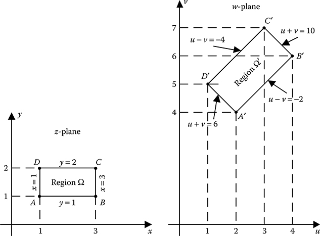
FIGURE 11.3
Pertaining to Problem 11.1.

PROBLEM 11.2

Let Ω be the rectangular region in the z-plane bounded by x = 1, y = 1, x = 3 and y = 2. Find the mapped region Ω’ in the w-plane under the linear transformation w = (1 + i)z + (2 + 2i).

Solution:

Given, w = f(z) = (1 + i)z + (2 + 2i) = (1 + i)(x + iy) + (2 + 2i) = (x − y + 2) + i (x + y + 2).

Hence, u = x − y + 2 and v = x + y + 2.

Therefore, for x = 1, u = − y + 3 and v = y + 3 or, u + v = 6, that is, the line x = 1 in the z-plane is mapped to the straight line u + v = 6 in the w-plane.

Similarly, for y = 1, u = x + 1 and v = x + 3 or, u − v = −2.

For x = 3, u = − y + 5 and v = y + 5 or, u + v = 10.

For y = 2, u = x and v = x + 4 or, u − v = −4.

Therefore, the four straight lines in the z-plane defined by x = 1, y = 1, x = 3 and y = 2 are mapped to four straight lines defined by u + v = 6, u − v = −2, u + v = 10 and u − v = −4, respectively, in the w-plane. The mapping is shown in Figure 11.4. Under the linear transformation w = az + b, where a = 1 + i and b = 2 + 2i, it may be seen that the rectangular region Ω in the z-plane is translated by b(= 2 + 2i), rotated by an angle 45° [ = arg(a) = arg(1 + i)] in the anti-clockwise direction and dilated by √2(= |a| = |1 + i|) to another rectangular region Ω′ in the w-plane.

Images

FIGURE 11.4
Pertaining to Problem 11.2.

11.3 Concept of Complex Potential

Let, ϕ(x,y) be a harmonic function in a domain Ω. It is possible to define a harmonic conjugate function, ψ(x,y), uniquely by Cauchy–Riemann equations in the same domain. Thus, an analytic function of z = x + iy in the domain Ω can be written as

$F (z) = ϕ (x, y) + i ψ (x, y) (11.13)$

Consequently, F(z) conformally maps the curves in the z-plane onto the corresponding curves in the w-plane and vice versa preserving the angles during mapping.

Because both the real and imaginary parts of F(z), namely, ϕ(x,y) and ψ(x,y), are harmonic functions, they satisfy Laplace’s equation and hence either one of these two could be used to find potential. Thus, the complex analytic function F(z) is known as complex potential. Laplace’s equation is one of the most important partial differential equations in engineering and physics. The theory of solutions of Laplace’s equation is known as potential theory. The concept of complex potential relates potential theory closely to complex analysis.

If ϕ(x,y) is considered to be real potential, then ϕ(x,y) = const represents equipotential lines in the z-plane. Because ϕ(x,y) and ψ(x,y) are orthogonal, ψ(x,y) = const represents electric fieldlines in the z-plane. For example, consider the complex potential function as F(z) = Az + B = Ax + B + iAy. Then the equipotential lines corresponding to ϕ(x,y) = Ax + B = const are straight lines parallel to y-axis and the electric fieldlines corresponding to ψ(x,y) = Ay = const are straight lines parallel to x-axis.

Introduction of the concept of complex potential is advantageous in the following ways: (1) it is possible to handle equipotential and electric field-lines simultaneously and (2) Dirichlet problems with difficult geometry of boundaries could be solved by conformal mapping by finding an analytic function F(z), which maps a complicated domain Ω in the z-plane onto a simpler domain Ω’ in the w-plane. The complex potential F′(w) is solved in the w-plane by satisfying Laplace’s equation along with the boundary conditions. Then the complex potential in the z-plane can be obtained by inverse transform from which the real potential is obtained as ϕ(x,y) = Re[F(z)].

This is a practicable way of solution as harmonic functions remain harmonic under conformal mapping.

11.4 Procedural Steps in Solving Problems Using Conformal Mapping

Find an analytic function w = F(z) to map the original region Ω in the z-plane to the transformed region Ω′ in the w-plane. The region Ω′ should be a region for which explicit solutions to the problem at hand are known.
Transfer the boundary conditions from the boundaries of the region Ω in the z-plane to the boundaries of the transformed region Ω′ in the w-plane.
Solve the problem and find the complex potential F′(w) for the transformed region Ω′ in the w-plane.
Map the solution F′(w) for the region Ω′ in the w-plane back to the complex potential F(z) for the region Ω in the z-plane through inverse mapping.

The steps are schematically shown in Figure 11.5. The most important step is to find an appropriate mapping function w = F(z), which fits the problem at hand. Once the right mapping function has been found, the problem is as good as solved.

Images

FIGURE 11.5
Schematic representation of solution of potential problem by conformal mapping.

11.5 Applications of Conformal Mapping in Electrostatic Potential Problems

Conformal mapping is a powerful method for solving boundary value problems in a two-dimensional potential theory through the transformation of a complicated region into a simpler region. Electric potential satisfies Laplace’s equation in charge-free region. Therefore, electrostatic field that satisfies Laplace’s equation in a two-dimensional region in x–y plane, will also satisfy Laplace’s equation in any plane to which the region may be transformed by an analytic complex potential function F(z). For each value of complex z = x + iy, there is a corresponding value of complex w = F(z). In other words, for every point in the z-plane, there is a corresponding point in the w-plane. As a result, the locus of any point in the z-plane will trace another path in w-plane. Let the locus in the z-plane maps onto a path ϕ′(u, v) = const in the w-plane, which corresponds to an equipotential and may also be the surface of a conductor. Then the problem can be solved in the w-plane incorporating the appropriate boundary condition, that is, the value of the conductor potential, and the results can be mapped back to z-plane to get the real potential and then the electric fieldlines can be obtained from the conjugate harmonic function. This section discusses some of the applications of conformal mapping in solving two-dimensional electrostatic potential problems.

11.5.1 Conformal Mapping of Co-Axial Cylinders

The cross-sectional view of a single-core cable is shown in Figure 11.6, where the co-axial cylindrical conductors are of infinite length in the direction normal to the plane of the paper. Hence, the field varies only in the cross-sectional plane and is translationally invariant in the direction of the length of the cable. Let the cross-sectional plane of the cable be the x–y plane or the z-plane. Then the field in the region between the two cylindrical conductors can be found by conformal mapping. Let the radii of the inner and the outer conductors be r₁ and r₂, respectively, and the potential of the inner and the outer conductors be V and zero, respectively.

Consider the complex analytical function for conformal mapping be

$w = u + i v = C_{1} \ln (z) + C_{2} (11.14)$

where, z = x + iy = re^iθ such that $r = \sqrt{x^{2} + y^{2}}$ and θ = tan⁻¹(y/x)

Therefore,

$\begin{matrix} u + i v = C_{1} \ln (r e^{i θ}) + C_{2} = C_{1} \ln r + C_{2} + i C_{1} θ \\ or, u = C_{1} \ln (r) + C_{2} and v = C_{1} θ \end{matrix} (11.15)$

For the inner conductor, $x^{2} + y^{2} = r_{1}^{2}$ and hence it maps to a straight line u₁ = constant parallel to v-axis in the w-plane. Similarly, the outer conductor for each $x^{2} + y^{2} = r_{2}^{2}$ maps to another straight line u₂ = constant parallel to v-axis in the w-plane, as shown in Figure 11.6. In other words, the field within the two cylindrical conductors in the z-plane is conformally mapped to field between two infinitely long parallel plates, that is, the field within a parallel plate capacitor, in the w-plane. From Figure 11.6 it may be seen that the orthogonality of the equipotentials in the form of circles and electric fieldlines in the form of radial lines in the z-plane are maintained in the w-plane, where the equipotentials are straight lines parallel to v-axis and the electric fieldlines are straight lines parallel to u-axis.

Images

FIGURE 11.6
Conformal mapping of co-axial cylinders.

From the boundary conditions on the conductor surfaces

$C_{1} \ln r_{1} + C_{2} = V (11.16)$

$and C_{1} \ln r_{2} + C_{2} = 0 (11.17)$

From Equations 11.16 and 11.17,

$C_{1} = - \frac{V}{\ln (r_{2} / r_{1})} and C_{2} = \frac{V \ln r_{2}}{\ln (r_{2} / r_{1})} (11.18)$

The potential at any radius r is given by u = C₁ ln r + C₂. Correspondingly, in the z-plane

$ϕ (x, y) = - \frac{V \ln r}{\ln (r_{2} / r_{1})} + \frac{V \ln r_{2}}{\ln (r_{2} / r_{1})} = \frac{V \ln (r_{2} / r)}{\ln (r_{2} / r_{1})} (11.19)$

Then,

$E_{r} (x, y) = - \frac{\partial ϕ}{\partial r} = \frac{V}{r \ln (r_{2} / r_{1})} (11.20)$

Equation 11.20 gives the value of electric field intensity at any radius r, which is the same as the one given by Equation 4.30.

11.5.2 Conformal Mapping of Non-Co-Axial Cylinders

Figure 11.7 shows two non-co-axial cylinders in the z-plane, such that for the outer cylinder C₂, |z| = 1. Radius of the inner cylinder C₁ is (1/5) and its centre is located at a distance of (1/5) from the centre of the larger cylinder. In this case also the length of the two cylinders is taken to be infinite in the direction normal to the plane of the paper. Hence, the field in the space between the two cylinders does not vary in the direction of the length of the cylinders. Therefore, the cross-sectional plane is shown to be the z-plane in Figure 11.7. The inner cylinder is at a potential of V while the outer cylinder is earthed. Direct solution of the field between the two cylinders is difficult in the z-plane. However, it is possible to conformally map the non-co-axial cylinders in the z-plane onto two co-axial cylinders in the w-plane keeping the boundary conditions, that is, boundary potentials, same.

In this transformation, the unit radius outer circle C₂ in the z-plane is mapped onto a unit radius circle $C_{2}^{'}$ in the w-plane in such a way that the inner circle $C_{1}^{'}$ becomes concentric with a radius r_i, as shown in Figure 11.7. The mapping function for this linear fractional transformation is

$w = \frac{z - k}{k z - 1} (11.21)$

Images

FIGURE 11.7
Conformal mapping of non-co-axial cylinders.

As shown in Figure 11.7, the two points on the inner circle A(0,0) and B(2/5, 0) in the z-plane are mapped onto two points A′(r_i,0) and B′(−r_i,0) on the inner circle in the w-plane.

Hence, from Equation 11.21 for the points A(0,0) and A′(r_i,0) r_i = (0 – k)/(0 − 1) = k and for the points B (2/5, 0) and B′(−r_i,0) –r_i = [(2/5) – k]/[(2k/5) – 1] = (2 − 5r_i)/(2r_i − 5) or, $r_{i}^{2} - 5 r_{i} + 1 = 0$ , or, r_i = 4.79 and 0.208.

But, r_i cannot be greater than 1 and hence, r_i = 0.208. Therefore, k = r_i = 0.208.

Thus, the mapping function for this problem is

$w = \frac{z - 0.2 08}{0.2 08 z - 1} (11.22)$

Writing the complex potential function in the w-plane as F′(w) = aln w + b, the real part of the complex potential can be written as

$ϕ' (u, v) = Re [F' (w)] = a \ln | w | + b (11.23)$

Two conditions on boundary potentials in the w-plane are as follows: (1) ϕ′ = 0 for |w| = 1 and (2) ϕ′ = V for |w| = r_i

Application of first boundary condition on Equation 11.23 yields

a ln1 + b = 0, or, b = 0

Similarly, applying the second boundary condition on Equation 11.23 one would get

a ln r_i + b = V, or ln 0.208 = V, or, a = −0.6368 V

Thus, the desired solution for complex potential in the z-plane is

$F (z) = - 0.6 368 V \ln \frac{z . - 0.2 08}{0. 208 z - 1} (11.24)$

The real potential within the two cylinders is then given by

$ϕ (x, y) = Re [F (z)] = - 0.6 368 V \ln | \frac{z . - 0.2 08}{0. 208 z - 1} | (11.25)$

If the potentials are +V and –V instead of V and 0, then from the first boundary condition

aln1 + b = −V, or b = −V

and from the second boundary condition aln r_i + b = V, or, aln0.208 − V = V or, a = −1.273 V.

Hence, the desired solution for complex potential in the z-plane is

$F (z) = - 1.2 73 V ln \frac{z . - 0.2 08}{0. 208 z - 1} - V = V (- 1.2 73 \ln \frac{z . - 0.2 08}{0. 208 z - 1} - 1) (11.26)$

The real potential within the two cylinders is then given by

$ϕ (x, y) = Re [F (z)] = V (- 1.2 73 \ln | \frac{z - 0.2 08}{0. 208 z - 1} | - 1) (11.27)$

11.5.3 Conformal Mapping of Unequal Parallel Cylinders

Figure 11.8 shows two unequal parallel cylinders in the z-plane, such that for the larger cylinder C₂, |z| = 1. Radius of the smaller cylinder C₁ is (1/2) and its centre is located at a distance of (7/2) from the centre of the larger cylinder. In this case also the length of the two cylinders is taken to be infinite in the direction normal to the plane of the paper. Hence, the field in the space between the two parallel cylinders does not vary in the direction of the length of the cylinders. Therefore, the cross-sectional plane is shown to be the z-plane in Figure 11.8. The smaller cylinder is at a potential of V whereas the larger cylinder is earthed. It is possible to map these two parallel cylinders onto two co-axial cylinders in the w-plane as follows.

In this transformation, too, the unit radius larger circle C₂ in the z-plane is mapped onto a unit radius circle $C_{2}^{'}$ in the w-plane in such a way that the smaller circle $C_{1}^{'}$ becomes concentric with a radius r_i, as shown in Figure 11.8. The mapping function for this linear fractional transformation is also

$w = \frac{z - k}{k z - 1} (11.28)$

Images

FIGURE 11.8
Conformal mapping of two unequal parallel cylinders.

However, as shown in Figure 11.8, the two points on the smaller circle A(3,0) and B(4,0) in the z-plane are mapped onto two points A′(−r_i,0) and B′(r_i,0) on the inner circle in the w-plane.

Hence, from Equation 11.26 for the points A(3,0) and A′(−r_i,0), −r_i = (3−k)/(3k − 1) and for the points B(4,0) and B′(r_i,0), r_i = (4 − k)/(4k − 1) = (k − 3)/(3k − 1) or, 7k² − 26k + 7 = 0, or, k = 3.42 and 0.292.

For k = 3.42, r_i = 0.046 and for k = 0.292, r_i = 21.84.

But r_i cannot be greater than 1 in the w-plane, so the solution is k = 3.42 and r_i = 0.046.

Writing the same complex potential function in the w-plane as F′(w) = alnw + b, as in Section 11.5.2, and applying the same boundary conditions for potential, as shown in Figure 11.8,

$b = 0 and a = \frac{V}{\ln r_{i}} = \frac{V}{\ln 0.0 46} = - 0.3 247 V$

Thus, the desired solution for complex potential in the z-plane is

$F (z) = - 0.3 247 V \ln \frac{z - 3.4 2}{3. 42 z - 1} (11.29)$

The real potential between the two unequal parallel cylinders is then given by

$ϕ (x, y) = Re [F (z)] = - 0.3 247 V \ln | \frac{z - 3.4 2}{3. 42 z - 1} | (11.30)$

If the potentials are +V and –V instead of V and 0, then from the first boundary condition

a ln 1 + b = −V, or b = −V

and from the second boundary condition a ln r_i + b = V, or, a ln 0.046 − V = V or, a = −0.6494 V.

Hence, the desired solution for complex potential in the z-plane is

$F (z) = - 0.6 494 V ln \frac{z - 3.4 2}{3. 42 z - 1} - V = V (- 0.6 494 \ln \frac{z - 3.4 2}{3. 42 z - 1} - 1) (11.31)$

The real potential between the two unequal parallel cylinders is then given by

$ϕ (x, y) = Re [F (z)] = V (- 0.6 494 \ln | \frac{z - 3.4 2}{3. 42 z - 1} | - 1) (11.32)$

11.5.3.1 Conformal Mapping of Equal Parallel Cylinders

With reference to Figure 11.8, if the radius of the cylinder 1, that is, C₁, is taken to be unity, then

k = 2.906 and r_i = 0.064

Hence, if the potentials of the two cylinders are V and 0, respectively, then the desired solution for complex potential in the z-plane is

$F (z) = - 0.3 638 V \ln \frac{z - 2.9 06}{2. 906 z - 1} (11.33)$

The real potential between the two equal parallel cylinders is then given by

$ϕ (x, y) = Re [F (z)] = - 0.3 638 V \ln | \frac{z - 2.9 06}{2. 906 z - 1} | (11.34)$

If the potentials of the two cylinders are +V and −V, respectively, then the desired solution for complex potential in the z-plane is

$F (z) = - 0.7 276 V ln \frac{z - 2.9 06}{2. 906 z - 1} - V = V (- 0.7 276 \ln \frac{z - 2.9 06}{2. 906 z - 1} - 1) (11.35)$

The real potential between the two equal parallel cylinders is then given by

$ϕ (x, y) = Re [F (z)] = V (- 0.7 276 \ln | \frac{z - 2.9 06}{2. 906 z - 1} | - 1) (11.36)$

Objective Type Questions

1. Conformal mapping could be used in

a. Two-dimensional system

b. Axi-symmetric system

c. Three-dimensional system

d. All the above

2. In conformal mapping, the angle between intersecting curves

a. Increases by 90°

b. Decreases by 90°

c. Increases by 180°

d. Remains the same

3. Both real and imaginary parts of the complex potential F(z) are harmonic functions. If Re[F(z)] = constant represents equipotential lines, then Imag[F(z)] = constant represents

a. Electric flux lines

b. Equipotential lines

c. Zero potential line

d. None of the above

4. In conformal mapping from z-plane to w-plane, which of the following operations are commonly performed?

a. Scaling

b. Rotation

c. Translation

d. All the above

5. By conformal mapping which of the following configurations in the z-plane could be mapped to co-axial cylinders in the w-plane?

a. Non-co-axial cylinders

b. Unequal parallel cylinders

c. Equal parallel cylinders

d. All the above

6. With the help of the complex analytic function w = a ln z + b, which of the following configuration in the z-plane could be mapped to parallel plate capacitor in the w-plane?

a. Co-axial cylinders

b. Parallel cylinders

c. Two equal spheres

d. None of the above

7. In conformal mapping, a real-life configuration is mapped from

a. z-plane to s-plane

b. s-plane to z-plane

c. z-plane to w-plane

d. s-plane to w-plane

8. During conformal mapping from z-plane to w-plane

a. Shape is preserved

b. Angle of intersection is preserved

c. Boundary conditions are preserved

d. Both (b) and (c)

9. In conformal mapping of electrostatic field, complex potential is defined as F(z) = ϕ(x,y) + i ψ(x,y). If ϕ(x,y) is known, then ψ(x,y) can be found from

a. Gauss’s law

b. Cauchy–Riemann equations

c. Divergence theorem

d. Uniqueness theorem

10. In conformal mapping of electrostatic field, complex potential is defined as F(z) = ϕ(x,y) + i ψ(x,y). Then Laplace’s equation is satisfied by

a. F(z)

b. ϕ(x,y)

c. ψ(x,y)

d. Both (b) and (c)

11. In conformal mapping, equipotential and electric flux lines can be handled simultaneously by the introduction of the concept of

a. Complex potential

b. Complex electric field intensity

c. Complex electric flux density

d. None of the above

12. In spite of having numerical techniques, conformal mapping is used for electrostatic field analysis because it

a. Can provide quicker solution to difficult problems

b. Can provide more accurate solutions to difficult problems

c. Can provide benchmark solutions for some problems which can be used for validation of numerical results

d. All the above

Answers:

1) a;

2) d;

3) a;

4) d;

5) d;

6) a;

7) c;

8) d;

9) b;

10) d;

11) a;

12) c

..................Content has been hidden....................

You can't read the all page of ebook, please click here login for view all page.

Table of Contents for 11. Conformal Mapping

Create new playlist

Sign In

Sign Up

PROBLEM 11.1

PROBLEM 11.2

Answers:

Table of Contents for
11. Conformal Mapping