
13
Numerical Computation of Electric Field
ABSTRACT In a high-voltage equipment, as a thumb rule, the cost of insulation increases with the cube of voltage rating. However, practical experience shows that insulation failure is the most frequent cause of major breakdown of electrical equipment. Hence, it is of paramount importance that the insulation in electrical equipment withstands the electric field stresses with adequate safety margin. For this purpose, it is necessary to determine the electric field distribution precisely. An inherent advantage of analytic solutions is the exactness. However, analytic solutions for the electric field are available only for problems having simple configurations. When the complexities of theoretical formulae make analytic solution extremely difficult, if not impossible, then one has to take resort to non-analytic methods. Graphical, experimental and analog methods are applicable to solve fewer problems, which have less complexity. With the advent of fast digital computers, numerical methods came into prominence. Numerical methods make it possible to solve practical problems, which are very complex in nature, when appropriate procedural steps are followed. Numerical methods are commonly based on the solutions of partial differential equations or integral equations with some analytic simplification for easy implementation.
The design of the insulation of high-voltage apparatus between phases and earth and also between the phases is based on the knowledge of electric field distribution and the dielectric properties of the combination of insulating materials used in the system. The principal aim is that the insulation should withstand the electric stresses with adequate reliability and at the same time the insulation should not be over dimensioned. It is well known that the withstand voltage of the external insulation of apparatus designed with non-self restoring insulation is determined by the maximum value of electric field intensity within the insulation system. Further, corona discharges are eliminated by proper design of highvoltage shielding electrodes. Thus, a comprehensive study of the electric field distribution in and around high-voltage equipment is of great practical importance. High-voltage equipment, in practice, is, in most of the cases, subjected to AC field of frequency 50 or 60 Hz. These fields may be approximated as quasi-static as the wavelength is much longer compared to the dimension of the components involved. Because of this, the electrostatic field calculation is possible by the different methods in use. Mathematically, an electric field calculation problem may be formulated as follows. The purpose is to determine, at each point within the field region of interest (ROI), the value of potential ϕ(x,y,z) and that of the electric field intensity are to be determined, which are related as In order to do that, either Laplace’s equation for systems without any source of charge in the field region, or, Poisson’s equation for systems with sources of charge in the field region, are required to be solved. The solutions of these equations are called boundary value problems, whereby the boundary conditions are specified by means of the given potential of electrode (Dirichlet’s problem) or by the given value of electric field intensity (Neumann’s problem).
The methods that are employed for determination of electric field are detailed in Figure 13.1. The analytical methods can only be applied to the cases, where the electrode or dielectric boundaries are of simple geometrical forms such as cylinders, spheres and so on. In other words, in this method, the boundaries are required to be defined exclusively by known mathematical functions. The results obtained are very accurate. But, as it is obvious, this method cannot be applied to complex problems. However, the results obtained by analytical methods for standard configurations are used still today to validate the results obtained by some other approximate methods such as numerical methods. Earlier experimental as well as graphical methods were used to get a fair idea about the nature of field distribution in some practical cases. However, these methods are greatly limited in their areas of usage and the errors involved are usually very high for any complex problem to be taken directly for design purposes. FIGURE 13.1 Nowadays, in more and more engineering problems, it is found that it is necessary to obtain approximate numerical solutions rather than exact closed-form solutions. The governing equations and boundary conditions for these problems could be written without too much effort, but it may be seen immediately that no simple analytical solution can be found. The difficulty in these engineering problems lies in the fact that either the geometry or some other feature of the problem is irregular. Analytical solutions to this type of problems seldom exist; yet these are the kinds of problems that engineers need to solve. There are several alternatives to overcome this dilemma. One possibility is to make simplifying assumptions ignoring the difficulties to reduce the problem to one that can be easily handled. Sometimes this approach works; but, more often than not, it leads to serious inaccuracies. With the availability of computers today, a more viable alternative is to retain the complexities of the problem and find an approximate numerical solution. Several approximate numerical analysis methods have evolved over the years, as shown in Figure 13.1. For each practical field problem, depending on the dielectric properties, complexity of contours and boundary conditions, one or the other numerical method is more suited.
It states that once any method of solving Poisson’s or Laplace’s equations subject to given boundary conditions has been found, the problem has been solved once and for all. No other method can ever give a different solution. Proof: Consider a volume V bounded by a surface S. Also consider that there is a charge density ρv throughout V, and the value of the scalar electric potential on S is ϕs. Assume that there are two solutions of Poisson’s equation, namely, ϕ1 and ϕ2. Then Therefore, Now, each solution must also satisfy the boundary conditions. It is to be noted here that one particular point cannot have two different electric potentials, as the work done to move a unit positive charge from infinity to that point is unique. Let the value of ϕ1 on the boundary is ϕ1s and the value of ϕ2 on the boundary is ϕ2s and they must be identical to ϕs. Therefore, ϕ1s = ϕ2s = ϕs or ϕ1s − ϕ2s = 0 For any scalar ϕ and any vector , the following vector identity can be written. Consider the scalar as (ϕ1− ϕ2) and the vector as . Then from Iden tity 13.5, Now, integrating throughout V enclosed by S, Applying divergence theorem to the left-hand side of Identity 13.7, as ϕ1s = ϕ2s on the specified surface S. On the right-hand side of Identity 13.7, from Equation 13.4. Hence, Identity 13.7 reduces to Because cannot be negative, the integrand must be zero everywhere, so that the integral may be zero. Hence, Again, if the gradient of (ϕ1 − ϕ2) is zero everywhere, then This constant may be evaluated by considering a point on the boundary surface S, so that ϕ1 − ϕ2 = ϕ1s − ϕ2s = 0 or, ϕ1 = ϕ2 which means that the two solutions are identical. However, in practice, if the same problem is solved by using different numerical techniques, the results are not exactly the same. This is due to the fact that the errors in a particular numerical method are often problem dependent and hence the results are not exactly same in all the methods. Therefore, this is not a violation of the Uniqueness theorem.
The following are the procedural steps that need to be followed for most of the numerical electric field computation methods. At first, the ROI needs to be identified. ROI is the region where the solution for electric field is to be obtained. For example, normally the field solution is not needed within the electrode volume or below the earth surface. Hence, for an isolated electrode and the earth surface, the ROI will be a region between the electrode surface and the earth surface, as shown in Figure 13.2. Before the ROI is identified, the geometries of the components that comprise the field system need to be defined. This step is nowadays done with the help of computer-aided design (CAD) software. FIGURE 13.2 The subsequent procedural step is to discretize the entire ROI or the boundaries to create the nodes where the solution of field will be obtained. Ideally, one should find the field solution at each and every point within the ROI. But it will result in immense computational burden and hence the field solution is obtained at discrete nodes. This step is called discretization and is often done with the help of mesh generators, which are software modules that create the mesh within the entire ROI or on the boundaries. In order that the electric field solution can be obtained at any specific location within the ROI, a pre-defined variation of electric field between successive nodes is assumed. In fact, this assumption is a root cause of inaccuracy of the numerical method. FIGURE 13.3 The next step is to create the system of equations based on the numerical method that is being employed. Subsequently, the system of equations is solved using a suitable solver. The solver needs to be chosen depending on the nature of the coefficient matrix that is being created by the specific numerical method. This solution gives the results for the unknown field quantities at the predefined nodes. Finally, the results at any desired location is computed using the assumed variation of electric field between the nodes, which is termed as post-processing of results. The procedural steps are depicted in Figure 13.3.
1. Methods applicable to solve electric field problems having less complexity are a. Graphical method b. Experimental method c. Analytical method d. All the above 2. Numerical methods for the computation of electric field are commonly based on the solution of a. Partial differential equation b. Integral equation c. Both (a) and (b) d. None of the above 3. Design of the insulation of a high-voltage apparatus is based on the knowledge of a. Electric field distribution b. Magnetic field distribution c. Dielectric properties of insulating materials d. Both (a) and (c) 4. Power frequency electric field in a high-voltage apparatus could be approximated as quasi-static because a. The wavelength is much longer compared to the dimension of the components involved b. The wavelength is slightly longer compared to the dimension of the components involved c. The wavelength is slightly shorter compared to the dimension of the components involved d. The wavelength is much shorter compared to the dimension of the components involved 5. Boundary value problems where the boundary conditions are specified by means of the given value of electric potential are called a. Gauss’s problem b. Dirichlet’s problem c. Poisson’s problem d. Laplace’s problem 6. Boundary value problems where the boundary conditions are specified by means of the given value of electric field intensity are called a. Gauss’s problem b. Neumann’s problem c. Poisson’s problem d. Laplace’s problem 7. Results of numerical methods are commonly validated using the results obtained from a. Experimental method b. Analytical method c. Graphical method d. All the above 8. Accurate solutions of electric field problems having irregular geometries are obtained by a. Making simplifying assumptions ignoring the difficulties to reduce the problem b. Finding an approximate numerical solution by retaining the complexities of the problem c. Both (a) and (b) d. None of the above 9. According to uniqueness theorem, any electric field problem has been solved once and for all if particular equations subject to the given boundary conditions are solved, which are a. Gauss’s equation b. Laplace’s equation c. Poisson’s equation d. Both (b) and (c) 10. In numerical computation of electric field, the discretization of field region is carried out to a. Obtain field solution at each and every point within the field region b. Obtain field solution at discrete nodes within the field region c. Reduce the computational burden d. Both (b) and (c) 1) d; 2) c; 3) d; 4) a; 5) b; 6) b; 7) b; 8) b; 9) d; 10) d13.1 Introduction
13.2 Methods of Determination of Electric Field Distribution

Different methods for the determination of the electric field distribution.13.3 Uniqueness Theorem
13.4 Procedural Steps in Numerical Electric Field Computation
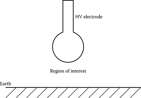
Depiction of the region of interest for electric field computation.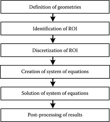
Procedural steps in numerical electric field computation.Objective Type Questions
Answers: