2. Gauss’s Law and Related Topics

Search in book...
Toggle Font Controls
Create new playlist

Name your new playlist

Playlist description (optional)
Sign In

Email address

Password

Forgot Password?

or

Continue with Facebook

Continue with Google
Sign Up

Full Name

Email address

Confirm Email Address

Password

or

Continue with Facebook

Continue with Google

ABSTRACT Gauss’s law constitutes one of the fundamental laws of electromagnetism. Gauss’s law provides an easy means of finding electric field intensity or electric flux density for symmetrical charge distributions such as a point charge, an infinite line charge, an infinite cylindrical surface charge and so forth. The procedure for applying Gauss’s law to calculate the electric field involves the introduction of Gaussian surfaces, which are closed surfaces on which electric field is either constant or zero. In most of the cases, electric field is either normal or tangential to the Gaussian surfaces. There are two different ways of stating Gauss’s law, namely, integral form and differential form, which are employed to solve field problems depending on suitability. These two forms of Gauss’s law in combination lead to divergence theorem. The divergence relationship between electric flux density and volume charge density as obtained from Gauss’s law and the gradient relationship between electric field intensity and electric potential could be combined in the form of an elliptic partial differential equation known as Poisson’s equation. In charge-free field region, Poisson’s equation reduces to Laplace’s equation. Both Poisson’s and Laplace’s equations could be solved for field quantities imposing suitable boundary conditions.

2.1 Introduction

German mathematician and physicist Karl Friedrich Gauss published his famous flux theorem in 1867, which is now well known in physics as Gauss’s law. It is one of the basic laws of classical field theory. Gauss’s law is a general law that can be applied to any closed surface. With the help of Gauss’s law, the amount of enclosed charge could be assessed by mapping the field on a surface outside the charge distribution. By the application of Gauss’s law, the electric field in many practical arrangements could be evaluated by forming a symmetric surface, commonly known as Gaussian surface, surrounding a charge distribution and then determining the electric flux through that surface.

In electric field theory, distinction is made between free charge and bound charge. Free charge implies a charge that is free to move over distances large as compared to atomic scale lengths. Free charge typically comes from electrons, for example, in the case of metals, or ions, or in the case of aqueous solutions. Bound charge implies charges of equal magnitude but opposite signs that are held close to each other and are free to move only through atomic scale lengths. Bound charges arise in the context of polarizable dielectric materials. Typical example of bound charge is the positive charge of an atomic nucleus and the negative charge of its associated electron cloud. The microscopic charge displacements in dielectric materials are not as dramatic as the rearrangement of charge in a conductor, but their cumulative effects account for the characteristic behaviour of dielectric materials. Typically, the detailed effect of bound charge is represented through electrical permittivity of dielectric materials, which will be discussed in Chapter 5. The Gauss’s law, as discussed in this chapter, is in terms of electric flux and the free charge only.

2.2 Useful Definitions and Integrals

2.2.1 Electric Flux through a Surface

Consider that the total electric flux through the surface S of an area A needs to be evaluated, as shown in Figure 2.1. The first important point to be noted here is that the electric flux density at different locations on S may not be the same. Therefore, the total flux through S has to be computed by subdividing the entire surface into a large number of smaller surfaces, such that over each small surface area, the electric flux density vector is uniform. As shown in Figure 2.1, for any small surface area dA, the area vector $d \vec{A}$ and the electric flux density vector $\vec{D}$ could be along different directions. Then the electric flux through dA is given by $\vec{D} \cdot d \vec{A}$

Then the total flux through S is given by the summation ${\vec{D}}_{1} \cdot d {\vec{A}}_{1} + {\vec{D}}_{2} \cdot d {\vec{A}}_{2} + \dots$

Images

FIGURE 2.1
Evaluation of the total electric flux through a surface.

When the sizes of the individual areas become infinitesimally small, then the total flux through S is given by the integral

$\int_{S} \vec{D} \cdot d \vec{A} = \iint \vec{D} \cdot d \vec{A} (2.1)$

2.2.2 Charge within a Closed Volume

Consider that the total charge within the volume V enclosed by the surface S needs to be evaluated, as shown in Figure 2.2. Here also, it is to be kept in mind that the distributed charge distribution may not be uniform throughout V. Then the entire volume needs to be subdivided into a large number of small volumes such that within each small volume, charge density is constant. Then the total charge within V is given by the summation ρ_v1dV₁ + ρ_v2dV₂ + ρ_v3dV₃ + …

When the sizes of the individual volumes become infinitesimally small, then the total charge within V is given by the integral ∫_Vρ_vdV = ∭ρ_vdV.

2.2.3 Solid Angle

The concept of solid angle is a natural extension of two-dimensional plane angle to three dimensions. The solid angle subtended by an area A at the point O is measured by the area Ω on the surface of the unit sphere centred at O, as shown in Figure 2.3. This is the area that would be cut out on the unit sphere surface by lines drawn from O to every point on the periphery of A. It is measured in terms of the unit called steradian, abbreviated as sr.

Consider an elementary area dA, as shown in Figure 2.4. If all the points on the periphery of dA are joined to the point O, then these lines cut out an area dΩ on the surface of the unit sphere. In other words, dA subtends a solid angle dΩ at O. Because the area is infinitesimally small, all points on dA could be considered to be equidistant from O. Let the distance of dA from O be r. The unit vector in the direction of the distance vector $\vec{r}$ is û_r. Because dA is infinitesimally small, it may be taken as flat for practical purposes and hence û_n is defined as the unit vector in the direction normal to dA, as shown in Figure 2.4. The angle between û_r and û_n is ϕ. Then the projection of dA on the sphere of radius r will be dS = dA cosϕ.

Images

FIGURE 2.2
Evaluation of the total charge within a volume.

Images

FIGURE 2.3
Solid angle subtended by an area at a point.

Images

FIGURE 2.4
Evaluation of the solid angle subtended by an elementary area.

The areas dS and dΩ have the same general shape and are related to the respective radii of the spheres having the following proportionality:

$\frac{d Ω}{d S} = \frac{1^{2}}{r^{2}}, or, d Ω = \frac{d A \cos ϕ}{r^{2}} = \frac{{\hat{u}}_{r} \cdot d \vec{A}}{r^{2}} (2.2)$

When an area completely encloses O, then Ω due to that area on the unit sphere will be 4π. Hence, the solid angle subtended at a point by an area that completely encloses the point is 4π sr, which happens to be maximum possible value of the solid angle.

2.3 Integral Form of Gauss’s Law

Gauss’s law states that the net electric flux through any closed surface enclosing a homogeneous volume of material is equal to the net electric charge enclosed by that closed surface. In other words, the surface integral of electric flux density vector over a closed surface is equal to the volume integral of charge densities within the volume enclosed by that surface.

In integral form,

$\int_{A} \vec{D} \cdot d \vec{A} = \int_{V} ρ_{v} d V (2.3)$

Gauss’s law is valid for any discrete set of point charges. Nevertheless, this law is also valid when an electric field is produced by charged objects with continuously distributed charges, because any continuously distributed charge may be viewed as a combination of discrete point charges.

Figure 2.5 shows a certain volume V of homogeneous material enclosed by a surface A. This volume is continuously charged by distributed charges. Consider these distributed charges to be represented by N number of discrete point charges, as shown in Figure 2.5.

Take a point charge q₁ located within V. Then consider an elementary area dA on A, as shown in Figure 2.5. The distance of dA from q₁ is, say, r.

Images

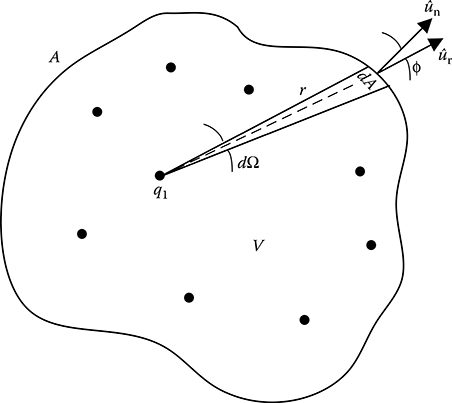
FIGURE 2.5
Pertaining to the integral form of Gauss’s law.

Then at a distance r from q₁,

${\vec{E}}_{1} = \frac{q_{1}}{4 π ε_{0} r^{2}} {\hat{u}}_{r} and {\vec{D}}_{1} = \frac{q_{1}}{4 π r^{2}} {\hat{u}}_{r} (2.4)$

Then, the total flux through A due to q₁ could be obtained as follows:

$\int_{A} {\vec{D}}_{1} \cdot d \vec{A} = \int_{A} \frac{q_{1}}{4 π} \frac{{\hat{u}}_{r} \cdot d \vec{A}}{r^{2}} = \frac{q_{1}}{4 π} \int_{A} d Ω, as \frac{{\hat{u}}_{r} \cdot d \vec{A}}{r^{2}} = d Ω (2.5)$

Because A completely encloses q₁, the solid angle subtended by A at the location of q₁ is 4π. Thus,

$\int_{A} {\vec{D}}_{1} \cdot d \vec{A} = \frac{q_{1}}{4 π} \times 4 π = q_{1} (2.6)$

Considering, N number of point charges within V, total electric flux density at the location of dA, as shown in Figure 2.5, will be as follows:

$\vec{D} = {\vec{D}}_{1} + {\vec{D}}_{2} + {\vec{D}}_{3} + ... + {\vec{D}}_{N} (2.7)$

Therefore, the total flux through A will be as follows:

$\begin{matrix} \int_{A} \vec{D} \cdot d \vec{A} & = \int_{A} ({\vec{D}}_{1} + {\vec{D}}_{2} + {\vec{D}}_{3} + ... + {\vec{D}}_{N}) \cdot d \vec{A} \\ = \int_{A} {\vec{D}}_{1} \cdot d \vec{A} + \int_{A} {\vec{D}}_{2} \cdot d \vec{A} + \int_{A} {\vec{D}}_{3} \cdot d \vec{A} + ... + \int_{A} {\vec{D}}_{N} \cdot d \vec{A} \\ = q_{1} + q_{2} + q_{3} + ... + q_{N} \end{matrix} (2.8)$

The right-hand side (RHS) of Equation 2.8 is equal to the total electric charge enclosed within V. Considering continuously distributed charge within V,

The total charge within is

$V = \int_{V} ρ_{v} d V$

where:

ρ_v is the volume charge density within V

Hence, Equation 2.8 can be rewritten as

$\int_{A} \vec{D} \cdot d \vec{A} = \int_{V} ρ_{v} d V$

From a physical viewpoint, the above expression indicates that the sum of all sources (positive electric charges) and all sinks (negative electric charges) within a volume gives the net flux through the surface enclosing the same volume.

Gauss’s law in integral form is only useful for exact solutions when the electric field has symmetry, for example, spherical, cylindrical or planar symmetry. The symmetry of the electric field follows from the symmetry of the charge distribution that is given. Therefore, the electric field of a symmetrically charged sphere will also have the spherical symmetry.

2.3.1 Gaussian Surface

A closed surface in a three-dimensional space through which the flux of a vector field is calculated is known as Gaussian surface. It is an arbitrary closed surface over which surface integral is performed to evaluate the total amount of enclosed source quantity, for example, electric charge. A Gaussian surface could also be used for calculating the electric field due to a given charge distribution.

Gaussian surfaces are normally carefully chosen in order to exploit symmetries to simplify the evaluation of the surface integral. If the symmetry is such that a surface can be found on which the electric field is constant, then the evaluation of electric flux can be done by multiplying the value of the field with the area of the Gaussian surface.

Two commonly used Gaussian surfaces are as follows:

The spherical Gaussian surface, which is chosen to be concentric with the charge distribution. It can be used to determine the electric field or electric flux due to a point charge or a spherical shell of uniform charge density or any other charge distribution with spherical symmetry, as shown in Figure 2.6.
The cylindrical Gaussian surface, which is chosen to be co-axial with the charge distribution. It can be used to determine the electric field or electric flux due to an infinitely long line of uniform charge density or an infinitely long cylinder of uniform charge density, as shown in Figure 2.7.

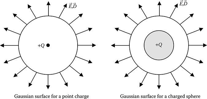
FIGURE 2.6
Spherical Gaussian surface.

FIGURE 2.7
Cylindrical Gaussian surface.

2.4 Differential Form of Gauss’s Law

If the electric field is known everywhere, then with the help of integral form of Gauss’s law, the charge in any given field region can be deduced by integrating the electric field. However, in most of the practical cases, the electric field needs to be computed when the electric charge distribution is known. This is much more difficult because even if the total flux through a given surface is known, the information about the electric field may be unknown, as electric flux could go in and out of the surface in complex patterns. In this context, the differential form of Gauss’s law becomes useful.

Consider that Gauss’s law is to be applied for the infinitesimal parallelepiped, as shown in Figure 2.8. The volume of the infinitesimal parallelepiped is ΔV = ΔxΔyΔz. Let the component of electric flux density going normally into the surface ABCD be D_y and that coming out of the surface EFGH be D_y + ΔD_y. Surfaces ABCD and EFGH are lying along the x–z plane. Then the net electric flux coming out in the y-direction, which is normal, to x–z plane is given by

Images

FIGURE 2.8
Application of Gauss’s law to a differential volume.

$(D_{y} + Δ D_{y}) Δ x Δ z - D_{y} Δ x Δ z = Δ D_{y} Δ x Δ z = \frac{Δ D_{y}}{Δ y} Δ x Δ y Δ z \approx \frac{\partial D_{y}}{\partial y} Δ V (2.9)$

Similarly, the net electric fluxes coming out in x- and z-directions are given by (∂D_x/∂x)ΔV and (∂D_z/∂z)ΔV, respectively. Hence, net electric flux coming of the volume ΔV

$= \frac{\partial D_{x}}{\partial x} Δ V + \frac{\partial D_{y}}{\partial y} Δ V + \frac{\partial D_{z}}{\partial z} Δ V = (\frac{\partial D_{x}}{\partial x} + \frac{\partial D_{y}}{\partial y} + \frac{\partial D_{z}}{\partial z}) Δ V$

Let ρ_v be the volume charge density of the small volume ΔV. Then according to Gauss’s law, the above expression for the net flux coming out of ΔV is equal to the total charge within the volume, that is, ρ_vΔV. Therefore,

$\begin{array}{l} (\frac{\partial D_{x}}{\partial x} + \frac{\partial D_{y}}{\partial y} + \frac{\partial D_{z}}{\partial z}) Δ V = ρ_{v} Δ V \\ or, \frac{\partial D_{x}}{\partial x} + \frac{\partial D_{y}}{\partial y} + \frac{\partial D_{z}}{\partial z} = ρ_{v} \end{array} (2.10)$

Equation 2.10 is known as the differential form of Gauss’s law. It can be expanded as follows:

$(\frac{\partial}{\partial x} \hat{i} + \frac{\partial}{\partial y} \hat{i} + \frac{\partial}{\partial z} \hat{k}) (D_{x} \hat{i} + D_{y} \hat{i} + D_{z} \hat{k}) = ρ_{v}, or, \vec{\nabla} \cdot \vec{D} = ρ_{v} (2.11)$

In Section 1.7.4, it has been mentioned that when the $\vec{\nabla}$ operator acts on a scalar quantity, it is denoted as gradient. As depicted in Equation 2.11, when the $\vec{\nabla}$ operator acts on a vector quantity with a dot product, then it is denoted as divergence.

The physical meaning of divergence of a vector field can be explained from the left-hand side (LHS) of Equation 2.10. From the above discussion, it may be seen that the LHS of Equation 2.10 is the net flux coming out per unit volume at a given location. Consequently, the divergence of a vector field at any location is the net flux of that vector field coming out per unit volume at that given location. If the divergence of a vector field is positive at any location, then the flux coming out of unit volume is higher than the flux going into the unit volume at that location. On the other hand, if the divergence of a vector field is negative, then the flux going into the unit volume is higher than the flux coming out of the unit volume.

2.5 Divergence Theorem

Integral form of Gauss’s law is, $\int_{A} \vec{D} \cdot d \vec{A} = \int_{V} ρ_{v} d V$ and differential form of Gauss’s law is, $\vec{\nabla} \cdot \vec{D} = ρ_{v}$ .

By substituting ρ_v on the RHS of the integral form by the LHS of the differential form, the above two equations could be combined as follows:

$\int_{A} \vec{D} \cdot d \vec{A} = \int_{V} (\vec{\nabla} \cdot \vec{D}) d V (2.12)$

where:

The volume V is enclosed by the surface A

Equation 2.12 shows that the divergence theorem could be used to convert a volume integral over V to a surface integral over A enclosing V.

2.6 Poisson’s and Laplace’s Equations

A useful approach to the calculation of electric potentials is to relate electric potential to electric charge density, which causes electric potential. Because electric potential is a scalar quantity, this approach has advantages over calculation of electric field intensity, which is a vector quantity. Once electric potential has been determined, the electric field intensity can be computed by taking the spatial gradient of electric potential.

The relationship between electric flux density and electric charge density is given by the differential form of Gauss’s law, that is, $\vec{\nabla} \cdot \vec{D} = ρ_{v}$ .

For homogeneous medium having uniform dielectric permittivity throughout the volume, the electric flux density and electric field intensity are related as $\vec{D} = ε \vec{E}$ .

The above two equations could be combined as follows:

$\vec{\nabla} \cdot (ε \vec{E}) = ρ_{v}, or, ε \vec{\nabla} \cdot \vec{E} = ρ_{v}, or, \vec{\nabla} \cdot \vec{E} = \frac{ρ_{v}}{ε} (2.13)$

Further, electric field intensity and electric potential are related as $\vec{E} = - \vec{\nabla} ϕ$ . Hence, from Equation 2.13, it may be written that

$\vec{\nabla} \cdot (- \vec{\nabla} ϕ) = \frac{ρ_{v}}{ε}, or, \vec{\nabla} \cdot \vec{\nabla} ϕ = - \frac{ρ_{v}}{ε}, or, {\vec{\nabla}}^{2} ϕ = - \frac{ρ_{v}}{ε} (2.14)$

Equation 2.14 is a partial differential equation of elliptic form and is named after the French mathematician Siméon Denis Poisson. Thus, it is commonly known as Poisson’s equation.

In Equation 2.14, the mathematical operation, the divergence of gradient of a function $(\vec{\nabla} \cdot \vec{\nabla} = {\vec{\nabla}}^{2})$ , is called the Laplacian, such that

${\vec{\nabla}}^{2} = (\frac{\partial}{\partial x} \hat{i} + \frac{\partial}{\partial y} \hat{j} + \frac{\partial}{\partial z} \vec{k}) . (\frac{\partial}{\partial x} \hat{i} + \frac{\partial}{\partial y} \hat{j} + \frac{\partial}{\partial z} \vec{k}) = \frac{\partial^{2}}{\partial x^{2}} + \frac{\partial^{2}}{\partial y^{2}} + \frac{\partial^{2}}{\partial z^{2}} (2.15)$

Therefore, Equation 2.14 can be written as follows:

$\frac{\partial^{2} ϕ}{\partial x^{2}} + \frac{\partial^{2} ϕ}{\partial y^{2}} + \frac{\partial^{2} ϕ}{\partial z^{2}} = - \frac{ρ_{v}}{ε} (2.16)$

Expressing the Laplacian in different coordinate systems to take advantage of the symmetry of a charge distribution simplifies the solution for the electric potential in many cases.

In electrostatic field problems, the dielectric media may be considered to be ideal insulation. In such case, free charges reside only on the conductor boundaries. Hence, the volume charge density (ρ_v) within the field region is zero. Then Equation 2.14 reduces to

${\vec{\nabla}}^{2} ϕ = 0, or, \frac{\partial^{2} ϕ}{\partial x^{2}} + \frac{\partial^{2} ϕ}{\partial y^{2}} + \frac{\partial^{2} ϕ}{\partial z^{2}} = 0, \frac{\partial^{2} ϕ}{\partial x^{2}} + \frac{\partial^{2} ϕ}{\partial y^{2}} + \frac{\partial^{2} ϕ}{\partial z^{2}} = 0 (2.17)$

Equation 2.17 is a second-order partial differential equation named after French mathematician Pierre-Simon Laplace and is commonly known as Laplace’s equation. There are an infinite number of functions that satisfy Laplace’s equation and the proper solution is found by specifying the appropriate boundary conditions, which will be discussed in Chapter 6.

In real-life problems, however, the dielectric media are never ideal dielectrics. Hence, there could be volume leakage as well as surface-leakage currents. Moreover, there could be discharges occurring within a particular zone of the insulation or there may be space charges that have accumulated over time within the field region of interest. In all such cases, volume charge density will be non-zero and hence Poisson’s equation needs to be solved to get the correct results.

2.7 Field due to a Continuous Distribution of Charge

The electric potential at a point p due to a number of discrete charges could be obtained as simple algebraic superposition of the electric potentials produced at p by each of discrete charges acting in isolation. If q₁,q₂,q₃,…,q_n are discrete charges located at distances r₁,r₂,r₃,…,r_n, respectively, from p, then the electric potential at p is given by

$ϕ_{p} = \frac{q_{1}}{4 π ε r_{1}} + \frac{q_{2}}{4 π ε r_{2}} + ... + \frac{q_{N}}{4 π ε r_{N}} = \frac{1}{4 π ε} \sum_{i = 1}^{N} \frac{q_{i}}{r_{i}} (2.18)$

Now, if the charges are distributed continuously throughout the field region, instead of being located at discrete number of points, the field region can be divided into large number of small elements of volume ΔV, such that each element contains a charge ρ_vΔV, where ρ_v is the volume charge density of the small element ΔV. The potential at a point p will then be given by

$ϕ = \frac{1}{4 π ε} \sum_{i = 1}^{N} \frac{ρ_{v i} Δ V_{i}}{r_{i}} (2.19)$

where:

r_i is the distance of the ith volume element from p

As the size of volume element becomes very small, the summation becomes an integration, that is,

$ϕ = \frac{1}{4 π ε} \int_{V} \frac{ρ_{v} d V}{r} (2.20)$

The integration is performed over the volume where the volume charge density has finite value. However, it must be noted here that it is not valid for charge distribution that extends to infinity.

Equation 2.20 is often written in the form

$ϕ = \int_{V} ρ_{v} G d V (2.21)$

In Equation 2.21, the function G = 1/4πε r is the potential due to a unit point charge and is often referred to as the electrostatic Green’s function for an unbounded homogeneous region.

2.8 Steps to Solve Problems Using Gauss’s Law

Typical steps that are often taken while solving electrostatic problems with the help of Gauss’s law are as follows:

An appropriate Gaussian surface with symmetry is selected that matches the symmetry of the charge distribution.
The Gaussian surface is so chosen that the electric field is either constant or zero at all points on the Gaussian surface.
The direction of $\vec{E}$ on the Gaussian surface is determined using the symmetry of field.
The surface integral of electric flux is computed over the selected Gaussian surface.
The charge enclosed by the Gaussian surface is determined from the surface integral. Solution for $\vec{E}$ is found.

PROBLEM 2.1

The potential field at any point in a space containing a dielectric material of relative permittivity 3.6 is given by ϕ = (3x²y − 2y²z + 5xyz²)V, where x,y,z are in metres. Calculate the volume charge density at the point P(5,3,2)m.

Solution:

$\begin{matrix} E_{x} = - \frac{\partial ϕ}{\partial x} = (- 6 x y - 5 y z^{2}) V / m, or, D_{x} = ε_{r} ε_{0} E_{x} C / m^{2} \\ E_{y} = - \frac{\partial ϕ}{\partial y} = (- 3 x^{2} + 4 y z - 5 x z^{2}) V / m, or, D_{y} = ε_{r} ε_{0} E_{y} C / m^{2} \\ E_{z} = - \frac{\partial ϕ}{\partial z} = (2 y^{2} - 10 x y z) V / m, or, D_{z} = ε_{r} ε_{0} E_{z} C / m^{2} \end{matrix}$

Therefore, $\frac{\partial D_{x}}{\partial x} = - 6 y ε_{r} ε_{0}, \frac{\partial D_{y}}{\partial y} = 4 z ε_{r} ε_{0} and \frac{\partial D_{z}}{\partial z} = - 10 x y ε_{r} ε_{0}$
Therefore, $ρ_{v} = \frac{\partial D_{x}}{\partial x} + \frac{\partial D_{y}}{\partial y} + \frac{\partial D_{z}}{\partial z} = (- 6 y + 4 z - 10 x y) ε_{r} ε_{0} C / m^{3}$

Hence, at the point P(5,3,2),

ρ_vP = −160 × 3.6 × 8.854 × 10⁻¹² = −5.1 nC/m³

PROBLEM 2.2

The electric flux density in free space is given by $\vec{D} = e^{- y} (\cos x \hat{i} - \sin x \hat{j}) C / m^{2}$ . Prove that the field region is charge free, that is, no free charge is present in the field region.

Solution:

It is required to be proved that ρ_v is zero in the field region. The given expression for electric flux density vector indicates that it is a case of two-dimensional field.

As given,

D_x = e^−y cos x and D_y = e^−y sin x

Hence,

$\frac{\partial D_{x}}{\partial x} = - e^{- y} \sin x and \frac{\partial D_{y}}{\partial y} = e^{- y} \sin x$

Therefore,

$ρ_{v} = \frac{\partial D_{x}}{\partial x} + \frac{\partial D_{y}}{\partial y} = - e^{- y} \sin x + e^{- y} \sin x = 0$

Thus, it is proved that no free charge is present in the field region.

PROBLEM 2.3

A sphere of radius R carries a volume charge density ρ_v(r) = kr, where r is the radial distance from the centre and k is a constant. Determine the electric field intensity inside and outside the sphere.

Solution:

Inside the sphere, at any radius r_i, the amount of charge enclosed is given by

$q (r_{i}) = \int_{0}^{γ_{i}} k r \frac{4 π}{3} r^{3} d r = \frac{4 π k}{3} \int_{0}^{γ_{i}} r^{4} d r = \frac{4 π k r_{i}^{5}}{15}$

Therefore, considering a spherical Gaussian surface of radius r_i (<R) within the given sphere, the electric flux is normal to the Gaussian surface and electric field intensity E_i(r_i) is constant over the Gaussian surface. Thus, applying Gauss’s law,

$ε_{0} \int {\vec{E}}_{i} (r_{i}) \cdot d \vec{A} = q (r_{i}), or, ε_{0} 4 π r_{i}^{2} E_{i} (r_{i}) = \frac{4 π k r_{i}^{5}}{15}, or, E_{i} (r) = \frac{k r_{i}^{3}}{15 ε_{0}}$

Because the electric field is directed radially, its vector form is

${\vec{E}}_{i} (r_{i}) = (\frac{k r_{i}^{3}}{15 ε_{0}}) {\hat{u}}_{r}$

Again, total charge within the sphere of radius R is (4πkR⁵)/15.

Hence, considering a spherical Gaussian surface of radius r_o(>R) outside the given sphere, the electric flux is again normal to the Gaussian surface and electric field intensity E_o(r_o) is constant over the Gaussian surface. Thus, applying Gauss’s law,

$ε_{0} 4 π r_{o}^{2} E_{o} (r_{o}) = \frac{4 π k R^{5}}{15}, or, E_{o} (r_{o}) = \frac{k R^{5}}{15 ε_{0} r_{o}^{2}}$

Because the electric field is directed radially, its vector form is

${\vec{E}}_{o} (r_{o}) = (\frac{k R^{5}}{15 ε_{0} r_{o}^{2}}) \hat{u} r$

PROBLEM 2.4

The electric flux density vector in a field region is given by $\vec{D} = (2 y + z) \hat{i} + 3 x y \hat{j} + 2 x \hat{k} C / m^{2}$ . Determine the total charge enclosed by the cube defined by 0 ≤ x ≤ 1, 0 ≤ y ≤ 1 and 0 ≤ z ≤ 1.

Solution:

According to Gauss’s law, the total charge enclosed by the cube will be equal to net flux through the cube (Figure 2.9).

For x = 0, the flux going into the cube through y–z plane, $\int_{0}^{1} \int_{0}^{1} (2 y + z) d y d z$ .

Again, for x = 1, the flux coming out of the cube through y–z plane, $\int_{0}^{1} \int_{0}^{1} (2 y + z) d y d z$ .

Because these two integrals are same, the net flux coming out of the cube in x-direction, that is, through y–z plane, is zero.

For y = 0, the flux going into the cube through x–z plane, $\int_{0}^{1} \int_{0}^{1} 3 x y d x d z = (3 y / 2) |_{y = 0} = 0$ .

For y = 1, the flux coming out of the cube through x–z plane, $\int_{0}^{1} \int_{0}^{1} 3 x y d x d z = (3 y / 2) |_{y = 1} = 1.5 C$ .

Therefore, the net flux coming out of the cube in y-direction, that is, through x–z plane is 1.5 C.

Images

FIGURE 2.9
Pertaining to Problem 2.4.

For z = 0, the flux going into the cube through x–y plane, $\int_{0}^{1} \int_{0}^{1} 2 x d x d z$ .

Again, for z = 1, the flux coming out of the cube through x–y plane, $\int_{0}^{1} \int_{0}^{1} 2 x d x d y$ .

Because these two integrals are same, the net flux coming out of the cube in z-direction, that is, through x–y plane, is zero.

Therefore, considering all three directions, net flux coming out of the cube is 1.5 C.

Hence, the total charge enclosed by the given cube is also 1.5 C.

PROBLEM 2.5

A cylinder of unit volume is placed in a uniform field with its axis parallel to the direction of field. Determine the total charge enclosed by the unit cylinder.

Solution:

On the curved surface of the cylinder, the direction of the area vector is radially outwards and hence is perpendicular to the electric field intensity, which is directed along the axis of the cylinder. Hence, on the curved surface $\int_{A} ε_{0} \vec{E} \cdot d \vec{A} = 0$ , that is, net flux through the curved surface of the cylinder will be zero.

As shown in Figure 2.10, the two end surfaces of the cylinder S1 and S2 are normal to the direction of electric field intensity. Thus, the electric flux going into the cylinder through the surface S1 on the LHS will be $ε_{0} | \vec{E} | A$ , where A is the area of S1. Similarly, the electric flux coming out of the cylinder through the surface S2 on the RHS will also be $ε_{0} | \vec{E} | A$ , as the area of S2 is also A. Because the field is stated to be uniform, electric field intensity is same everywhere. Therefore, the net flux through the end surfaces of the cylinder is also zero.

Images

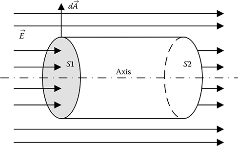
FIGURE 2.10
Pertaining to Problem 2.5.

Thus, the net flux through the cylinder considering all the surfaces of the cylinder is zero.

Hence, the total charge enclosed by the cylinder is zero.

Objective Type Questions

1. The potential field in free space is given by ϕ = (3xy − 4yz + 5zx)V, where x,y,z are in metres. At the point P(1,1,1)m, which one of the following is true?

a. Electric potential is zero

b. Electric field intensity is zero

c. Electric flux density is zero

d. Volume charge density is zero

2. Net electric flux through a closed surface enclosing a volume is equal to the sum of

a. Free charges and bound charges within the volume

b. Free positive charges within the volume

c. Free negative charges within the volume

d. Free positive and negative charges within the volume

3. On the Gaussian surface, electric field

a. Is constant at all points

b. Is zero at all points

c. Both (a) and (b)

d. Varies linearly

4. Solution for electric potential is commonly obtained by solving

a. Integral form of Gauss’s law

b. Differential form of Gauss’s law

c. Poisson’s equation

d. The equation derived from the divergence theorem

5. If the divergence of electric flux density through a unit volume is zero, then

a. The flux going into the volume is zero

b. The flux coming out of the volume is zero

c. Both the fluxes going in and coming out of the volume are zero

d. The difference between the fluxes going in and coming out of the volume is zero

6. Solution for electric potential in charge-free field region is obtained by solving

a. Laplace’s equation

b. Poisson’s equation

c. Integral form of Gauss’s law

d. Differential form of Gauss’s law

7. A volume integral can be converted to a surface integral and vice versa with the help of

a. Differential form of Gauss’s law

b. Divergence theorem

c. Poisson’s equation

d. Laplace’s equation

8. If the flux coming out of a closed surface enclosing a volume is higher than the flux going into the surface, then within the volume enclosed by the surface

a. Free positive charges are greater than free negative charges

b. Free positive charges are lesser than free negative charges

c. Free positive charges are greater than bound negative charges

d. Free positive charges are lesser than bound negative charges

9. For a closed surface enclosing a certain volume, Gauss’s law relates to

a. Free charge within the volume and electric potential on the surface

b. Both free and bound charges within the volume and electric potential on the surface

c. Free charge within the volume and electric flux through the surface

d. Both free and bound charges within the volume and electric flux through the surface

10. Which one of the following statements is not true?

a. Gauss’s law is valid for a set of discrete point charges

b. Gauss’s law in not valid for continuously distributed charges

c. Volume charge density is zero for charge-free field region

d. Divergence theorem can be obtained from integral and differential forms of Gauss’s law

Answers:

1) d;

2) d;

3) c;

4) c;

5) d;

6) a;

7) b;

8) a;

9) c;

10) b

..................Content has been hidden....................

You can't read the all page of ebook, please click here login for view all page.

Table of Contents for 2. Gauss’s Law and Related Topics

Create new playlist

Sign In

Sign Up

PROBLEM 2.1

PROBLEM 2.2

PROBLEM 2.3

PROBLEM 2.4

PROBLEM 2.5

Answers:

Table of Contents for
2. Gauss’s Law and Related Topics