
16
Numerical Computation of High-Voltage Field by Charge Simulation Method
ABSTRACT An alternative approach towards solving Laplace’s or Poisson’s equations by differential equation techniques is to take integrals of these equations using discrete charges or by subdividing the interfaces into subsections of charges. Conventional charge simulation method (CSM) is based on the usage of discrete charges. This chapter discusses in detail the simulation of single-dielectric as well as multi-dielectric arrangements using CSM for both symmetric and asymmetric systems. Different types of charge configurations, accuracy criteria and the factors affecting simulation accuracy have been presented at length. Formulations incorporating complex charges for computing field in systems having potentials with time-phase differences or for computing capacitive-resistive fields including volume, as well as surface, conductions has been thoroughly discussed. As the insulation in high-voltage equipment is often stressed by transient excitations, such cases have also been critically examined. Developments that have taken place over the years to improve the performance of CSM have also been included in this chapter. Two-dimensional, axi-symmetric as well as three-dimensional case studies of practical significance have been explained for the proper understanding of the simulation technique.
The principle of finite difference method (FDM) and finite element method (FEM) is to provide the entire region of interest (ROI) into a large number of sub-regions, and solve for unknown potentials a set of coupled simultaneous linear equations, which approximate Laplace’s or Poisson’s equations. Compared to these two methods, only boundary surfaces, that is, electrode surfaces and dielectric interfaces, are subdivided and charges are taken as unknowns in charge simulation method (CSM). First, it follows that the amount of human time and effort needed for subdivision is greatly reduced in CSM. Second, the electric field strength can be given explicitly in CSM without any numerical differentiation of the potential, which results in significant reduction in error. The second characteristic is very important because the field strength is usually more important for the design of an insulating system than electric potential. The earlier attempts for numerical field solutions employing CSM were reported by Loeb et al. in 1950 and then by Abou-Seada and Nasser [1]. Subsequently, in a comprehensive paper Singer, Steinbigler and Weiss presented the details of CSM [2]. Since then, many refinements to the original method have been proposed and CSM has evolved into a very powerful and efficient tool for computing electric fields in HV equipment. CSM is very simple and is applicable to systems having more than one dielectric medium. This method is also suitable for three-dimensional (3D) fields with or without symmetry.
The basic principle of conventional CSM is very simple. For the calculation of electric fields, the distributed charges on the surface of the electrode are replaced by N number of fictitious charges placed inside the electrode, as shown in Figure 16.1. The fictitious charges are placed inside the electrode to avoid singularity problem. In general, the fictitious charges are to be always placed outside the ROI, as the field is ideally required to be determined at all the points within the ROI. If the fictitious charges are placed within the ROI, then at the location of the fictitious charges singularity arises because at these points, the distance between the charge and the point at which the field solution is required becomes zero. FIGURE 16.1 The types and positions of these fictitious charges are predetermined, that is, user defined, but their magnitudes are unknown. In order to determine their magnitude, some collocation points, which are called contour points, are selected on the surface of electrode. In the conventional CSM, the number of contour points is chosen to be equal to the number of fictitious charges. Then it is required that at any one of these contour points the potential resulting from superposition of effects of all the fictitious charges is equal to the known electrode potential. Let Qj be the jth fictitious charge and ϕ be the known potential of the electrode. Then according to the superposition principle, where: Pij is the potential coefficient, that is, the potential at the point i due to a unit charge at the location j, which can be evaluated analytically for different types of fictitious charges by satisfying Laplace’s equation When Equation 16.1 is applied to N number of contour points, it leads to the following system of N linear equations for N unknown fictitious charges: In matrix form, Equation 16.2 can be written as where: [P] = potential coefficient matrix [ϕ] = column vector of known potential of contour points Equation 16.3 is solved for the unknown fictitious charges. As soon as the required fictitious charge system is determined, the potential and the field intensity at any point within the ROI can be calculated. Although the potential is found by Equation 16.1, the electric field intensities are calculated by superposition of all the stress vector components. For example, in the Cartesian co-ordinate system, the three superimposed field components at any point i are given as follows. where: Fx,ij, Fy,ij and Fz,ij are the electric field intensity coefficients in the x, y and z directions, respectively, that is, the components in the x, y and z directions, respectively, of electric field intensity at the point i for a unit charge at the location j In many cases, the effect of the ground plane is to be considered for electric field calculation. This plane can be taken into account by the introduction of image charge. Floating potential conductors are often present in high-voltage system, the most common example being condenser bushings. If floating electrodes are present, whose potentials are constant but unknown, then the boundary condition that is imposed for field computation is given below. Moreover, a supplementary condition is included such that the sum of fictitious charges for each floating electrode is zero. Then the system of equation that is obtained will be as follows: If the floating electrode has a net charge, then the supplementary condition is included such that the sum of its fictitious charges is equal to the known net charge value (QE). In Equation 16.8 the first row is then modified as follows
The field computation for multi-dielectric system is somewhat complicated due to the fact that the dipoles are realigned in dielectric media under the influence of the applied voltage. Such realignment of dipoles produces a net surface charge on the dielectric interface. Thus, in addition to the electrodes, each dielectric interface needs to be simulated by fictitious charges. Here, it is important to note that the dielectric boundary does not correspond to an equipotential surface. Moreover, it must be possible to calculate the electric field on both sides of the dielectric boundary. It has been mentioned earlier that the fictitious charges should be outside the ROI. In the case of electrodes this has been achieved by placing the charges within the electrodes. But, for the dielectric–dielectric interface, both the sides are within the ROI. Hence, any fictitious charge placed on either side of the interface would cause singularity problem. This issue is solved by placing two charges for every contour point on the dielectric–dielectric interface. For solving the field within the dielectric A, the set of charges placed within dielectric B are considered and vice versa. In the simple example shown in Figure 16.2, there are N1 number of charges and contour points to simulate the electrode, of which NA are on the side of dielectric A and (N1 − NA) are on the side of dielectric B. These N1 charges are valid for field calculation in both the dielectrics. At the dielectric interface, there are N2 contour points sequentially numbered from (N1 + 1, . . .,N1 + N2), with N2 charges (N1 + 1,. . .,N1 + N2) in dielectric A valid for dielectric B and N2 charges (N1 + N2 + 1,. . .,N1 + 2N2) in dielectric B valid for dielectric A. Altogether there are (N1 + N2) number of contour points and (N1 + 2N2) number of fictitious charges. FIGURE 16.2 In order to determine the fictitious charges, a system of equations is formulated by imposing the following boundary conditions. At each contour point on the electrode surface, the potential must be equal to the known electrode potential. This condition is also known as Dirichlet’s condition on the electrode surface. At each contour point on the dielectric interface, the potential and the normal component of flux density must be same when computed from either side of the boundary. Thus, the application of the first boundary condition to contour points 1 to N1 yields the following equations. Again, the application of the second boundary condition for potential and normal flux density to contour points N1 + 1 to N1 + N2 on the dielectric interface results in the following equations. From potential continuity condition: From continuity condition of normal flux density Dn: Equation 16.13 can be expanded as follows. where: Fn,ij is the field coefficient in the direction normal to the dielectric boundary at the respective contour point εA and εB are the permittivities of dielectrics A and B, respectively Equations 16.10 through 16.14 are solved to determine the unknown fictitious charges. These equations can be presented in matrix form, as shown in Matrix 16.M.1 Matrix 16.M.1 System of equations for CSM in multi-dielectric media.
The successful application of the CSM requires a proper choice of the types of fictitious charges. Point and line charges of infinite and semi-infinite lengths were used in the initial works on this method. Singer et al. [2] introduced ring charges and finite length line charges. Subsequently, a large variety of different charge configurations have been proposed. These other types of charge configurations include elliptic cylindrical charge, axi-spheroidal charge, plane-sheet charge, disk charge, ring-segment charge, volume charges, shell and annular plate charges as well as variable density line charge. In general, the choice of type of fictitious charge to be used depends on the complexity of the physical system and the available computational facilities. The potential and field coefficients for point and line charges are given by simple expressions and require very small computation time. For complex charge configuration, such coefficients may have to be computed numerically. On the other hand, a smaller number of charges may be used if complex charge configurations are employed, which reduces the overall memory requirement and computation time. In practice, most of the HV systems can be successfully simulated by using point, line and ring charges or a suitable combination of these charges. Point charge is the simplest of all types of fictitious charges. It can be used in two-dimensional (2D) as well as 3D configurations. Figure 16.3 shows the point charge Qj along with its image with respect to the x–y plane in 3D system. Then, the potential at the point i due to the point charge Qj and its image is given by where: FIGURE 16.3 Putting Qj = 1 in Equation 16.15, the expression for potential coefficient is given by Expressions for the electric field intensity coefficients are as follows: Infinite length line charges are used in 2D configurations, particularly for simulating long conductors in the case of transmission lines, cables and so on. Figure 16.4 shows the infinite length line charge Qj along with its image with respect to the x–z plane. In this configuration, electric field is considered to be independent of z-axis, that is, the length of the long conductors, while the field varies in the x–y plane, which is normal to the length of the long conductors. In a 2D system, all computations are performed for unit length of the system under consideration. Hence, Qj is the charge per unit length for the infinite length line charge. FIGURE 16.4 The expression for potential coefficient is then given by where: Expressions for the electric field intensity coefficients are as follows: Finite length line charges of uniform charge density are used in axi-symmetric configurations, particularly for simulating cylindrical geometries in the case of bushings, circuit breakers and so on. Figure 16.5 shows the finite length line charge along with its image. Finite length line charges of uniform charge density are commonly placed on the z-axis, that is, the axis of symmetry. Let the magnitude of the finite length line charge be Qj and the length of the charge be (zj2 − zj1), as shown in Figure 16.5. Then considering uniform charge density, charge per unit length is [Qj/(zj2 − zj1)]. The expressions for potential and electric field intensity coefficients were first developed by Steinbigler et al. [2] and are given below. FIGURE 16.5 The expression for potential coefficient is given by where: The expressions for the electric field intensity coefficients are as follows: FIGURE 16.6 Ring charges of uniform charge density are used in axi-symmetric configurations, particularly for simulating spherical- and cylindrical-shaped geometries. Figure 16.6 shows the ring charge along with its image. Ring charges of uniform charge density are commonly placed with their axes on the z-axis, that is, the axis of symmetry. Let the magnitude of the ring charge be Qj and the radius of the ring charge be rj, as shown in Figure 16.6. Then considering uniform charge density, charge per unit length is [Qj/(2πrj)]. The expressions for potential and electric field intensity coefficients were first developed by Singer et al. [2] and are given below. The expression for potential coefficient is given by where: K(k1) and K(k2) are elliptic integrals of first kind such that The expressions for the electric field intensity coefficients are as follows: where: E(k1) and E(k2) are elliptic integrals of second kind such that Arbitrary line segment charge having uniform charge density is used to simulate 3D geometries. Figure 16.7 shows an arbitrary line segment charge along with its image. Let the magnitude of the line segment charge be Qj and the length of the line segment charge be l, as shown in Figure 16.7. The expressions for potential and electric field intensity coefficients were first developed by Utmischi [3] and are given below. FIGURE 16.7 The expression for potential coefficient is given by In the development of this expression, the following coordinate transformations are carried out: (1) displacement of the origin to the points (xj, yj, zj) and (xj, yj, −zj); (2) rotation of Qj by α and −Qj by −α in the x–z plane and (3) rotation of Qj and −Qj by an angle β in the x–y plane. Thus, and The expressions for the electric field intensity coefficients are as follows: Differentiation of Pij in the coordinate systems (x1, y1, z1) and (x2, y2, z2) gives the electric field intensity coefficient components (Fx1,ij, Fy1,ij, Fz1,ij) and (Fx2,ij, Fy2,ij, Fz2,ij), respectively. Arbitrary ring segment charge having uniform charge density is used to simulate 3D geometries. Figure 16.8 shows an arbitrary ring segment charge along with its image. Let the magnitude of the line segment charge be Qj and the radius of the ring segment charge be r0, as shown in Figure 16.8. FIGURE 16.8 The expressions for potential and electric field intensity coefficients were first developed by Utmischi [3] and are given below. In the development of the expressions for potential and electric field coefficients, the following coordinate transformations are carried out: (1) displacement of the origin to the points (xj, yj, zj) and (xj, yj, −zj); (2) rotation of Qj by α and −Qj by −α in the x–z plane and (3) rotation of Qj and −Qj by an angle β in the x–y plane. Thus, the coordinate systems (x1, y1, z1) and (x2, y2, z2) are assigned to the ring segment charge Qj and its image −Qj, which are to be derived as per Equations 16.30 and 16.31, respectively. The expression for the potential coefficient is given as where: The electric field intensity components are determined as per Equation 16.32 where: (Fx2,ij, Fy2,ij, Fz2,ij) are determined in the same way for the image charge. Integrations are generally carried out numerically.
In order to calculate the field for a sinusoidal applied voltage, the calculations can be performed as a DC field in so far as the applied voltage does not change so fast that electromagnetic treatment is required. Then the instantaneous field strength is merely dependent on the applied voltage at that time instant. Thus, the conventional CSM with real fictitious charges can be used to compute AC fields for three-phase systems. It has been shown that the field distribution for sinusoidal applied voltage can be calculated in an efficient way by the use of complex fictitious charges. This is permitted because the fictitious charges also change sinusoidally with an angular frequency same as that of the applied voltage. Hence, by the use of complex fictitious charges, Equation 16.1 is modified as follows. where a bar on a variable represents a complex quantity. Application of Equation 16.34 to N number of contour points consists of a set of simultaneous linear equations for complex unknown charges with real coefficients as given below in matrix form. Equation 16.35 is solved to find complex solutions for the fictitious charges. To explain the above technique in a detailed manner, consider the case of Figure 16.9, which shows four conductors of which three are energized from a three-phase AC source, while the fourth one is grounded. Let Vph be the phase voltage of the three-phase source. Again, let there be N number of complex fictitious charges and contour points, respectively, for each conductor. The charges and the contour points are numbered as follows, 1,…,N for conductor A; N + 1,…,2N for conductor B; 2N + 1,…,3N for conductor C and 3N + 1,…,4N for conductor G. Then the application of Equation 16.34 to all these contour points gives the following equations. FIGURE 16.9 For conductor A: For conductor B: For conductor C: For conductor G: Equations 16.36 through 16.39 can be expressed in matrix form, as shown in Matrix 16.M.2: Matrix 16.M.2 System of equations for CSM application in three-phase conductor arrangement using complex fictitious charges. Matrix 16.M.2 is solved for the unknown complex fictitious charges .
Normally high-voltage equipment is insulated with materials of such a high resistivity that it can be treated as infinite for field calculation. In such cases, the field distribution is purely capacitive. But for lower values of volume or surface resistivity, the field distribution is capacitive-resistive or even resistive depending on the value of resistivity. In the case of capacitive field distribution, the instantaneous field is independent of waveform of applied voltage. But a very distinctive feature of capacitive-resistive fields is their time dependency and dependency on the waveform of applied voltage. Hence, capacitive-resistive field calculation including volume or surface resistivity is very important in studying DC and low frequency fields, impulse fields, contaminated insulators, voltage dividers, cables and so on. Bachmann [4] first proposed a technique based on CSM for capacitive-resistive field calculation. In his method, as the first step, the capacitive field distribution is calculated by CSM assuming resistivity to be infinite. Then the electrode–electrode and dielectric interface–electrode capacitances are calculated from this capacitive field distribution. After this, as the second step, an equivalent R-C network is constructed, which comprises these capacitances and surface resistances. Finally, the voltage distribution for the capacitive-resistive field is calculated from the R-C network. This method has two major drawbacks. First, the capacitances between the dielectric interface and electrode are dependent on the field distribution and hence, are not identical in capacitive and capacitive-resistive fields. Second, the calculation of field intensities from the R-C network is very laborious and results in significant errors. Takuma et al. [5] first proposed a method for direct simulation of the instantaneous capacitive-resistive field distribution with fictitious charges. Their method based on CSM and employing complex fictitious charges is generally extended, so that any capacitive-resistive field including volume resistance or surface resistance can be calculated, when the field distribution is Laplacian in the region except on the boundaries. Use of complex fictitious charges as well as appropriate boundary conditions permits the simulation of non-linear and transient problems also. Singer [6] has used complex charges and Fourier integrals to calculate the impulse stresses of conductive dielectrics. Use of discrete as well as area complex charges have been reported for capacitive-resistive field calculation. For capacitive-resistive field calculation including volume resistance, the principle of the method is that the field effect of the true charges produced by volume resistance is incorporated by means of complex fictitious charges in the CSM. If the volume charge density is σv, then where: is the electric field intensity Num erical Com putation of HV Field by Charge Simulation Method Again, if the current density through the volume of the dielectric is , then where: ρv is the volume resistivity and is constant, that is, independent of Now, if ε is independent of time t and E, then Equation 16.40 can be modified as follows: Equations 16.41 and 16.42 lead to For, AC fields of angular frequency ω, . Hence, Thus, Equation 16.43 can be rewritten as Equation 16.44 shows that the fields including volume resistivity εv can be computed by replacing the permittivity ε in purely capacitive field with the complex permittivity such that, where: Again, if is constant in the region of field calculation, then Equation 16.45 becomes Laplace’s equation as given below. Equation 16.45 permits the use of CSM for capacitive-resistive field calculation including volume resistance. However, from the above discussion, it becomes clear that in fields containing volume resistance, CSM cannot be applied to problems where ε or ρv is dependent on the electric field. This is because in such cases the field distribution cannot be expressed by superposing solutions of Laplace’s equation. The above method can be explained explicitly as described below. Consider a two-dielectric arrangement, as shown in Figure 16.10. In Figure 16.10, the two-dielectric media are assumed to have volume resistivities of ρvA and ρvB, respectively. The charges and the contour points are numbered in the same way as that given in Section 16.3. However, in Section 16.3, only real fictitious charges were taken for capacitive field calculation. But, for capacitive-resistive field calculation including volume resistance, complex fictitious charges are employed in place of real fictitious charges. The system of equations to be solved for unknown charges is derived by imposing the boundary conditions on the electrode surfaces and on the dielectric interfaces. The resulting equations with complex treatment are as follows. Dirichlet’s condition on the electrode surface: Equation 16.46 can be expanded for all the contour points on the electrode surface in the following way. FIGURE 16.10
Potential continuity condition on the dielectric interface: where: The subscripts A and B denote dielectrics A and B, respectively Equation 16.49 can be detailed explicitly as follows Continuity condition of Dn on the dielectric interface: where: Dn and σ represent normal component of electric flux density and surface charge density, respectively Equation 16.51 can also be written as Now, the surface current density at any point i on the dielectric interface due to volume resistance can be obtained as follows from Equation 16.53. For the case shown in Figure 16.11, is given by FIGURE 16.11 The surface charge density at any point i on the dielectric interface is given by Hence, Now, for AC fields of angular frequency ω, Therefore, Equation 16.54 can be rewritten as Thus, Equations 16.52 and 16.55 lead to where: Equation 16.57 is given below in details Equations 16.47, 16.48, 16.50 and 16.58 can be represented in matrix form as given below. Matrix 16.M.3 System of equations for capacitive-resistive field computation by CSM including volume resistance. It follows from Matrix 16.M.3, which is represented as Equation 16.59, that these are same as those for capacitive field, if the real values of the fictitious charges, permittivity, potential and field strength are replaced by their complex values. In fields including only surface resistance, true charges exist only on the boundary, that is, electrode and dielectric surfaces, and not inside the dielectric medium. As a result, the field distribution is always Laplacian inside each medium. This permits the application of CSM to capacitive-resistive field calculation, including surface resistance. The field distribution is obtained by superposing the effects of complex fictitious charges properly arranged inside the electrode and on both sides of the dielectric interface. The effect of true surface charges has to be incorporated into that of the complex fictitious charges. The method can be better explained by considering the two-dielectric arrangement shown in Figure 16.12. The difference is that, in this case, the volume resistivities of the two dielectrics are considered to be infinite and a uniform surface resistivities ρs is considered along the dielectric interface. The boundary conditions (1) and (2) as given by Equations 16.46 and 16.49, respectively, as well as the Equations 16.47, 16.48 and 16.50, in the case of volume resistance as given in sub-Section 16.6.1, are also valid in the case of surface resistance. However, the expression of surface charge density σ in continuity condition of , as given by Equation 16.51 in sub-Section 16.6.1, has to be modified as follows. In fields including surface resistance, the true surface charge density σ(i) is expressed as given below.
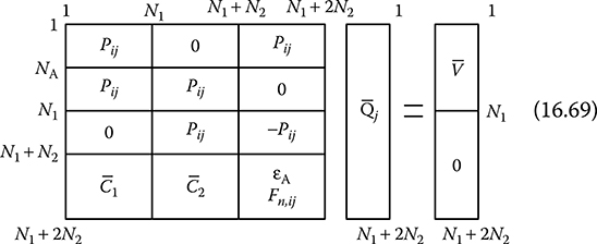
where: I(i) is the net surface current flowing into the ith contour point S(i) is a small surface area corresponding to that contour point For 2D or axi–symmetric cases, where the surface current I(i) flows in a predetermined direction, σ(i) can be expressed in terms of neighbouring potentials and resistances, as shown in Figure 16.13. where: R(i) and R(i + 1) are surface resistances corresponding to ith and (i + 1)th contour points, respectively, as shown in Figure 16.13 The expressions for R(i) and S(i) are detailed below. For 2D system (per unit length) FIGURE 16.12 FIGURE 16.13 For axi-symmetric system where: r′ is the r-coordinate of dl dl is a small length along the dielectric interface For AC fields of angular frequency ω, Equation 16.61 is modified as follows. Hence, from Equations 16.52 and 16.66, it follows that Equation 16.67 can be expressed explicitly as follows for the system of Figure 16.12. Now, the system of equations to be solved for unknown complex charges , as given by Equations 16.47, 16.48, 16.50 and 16.68, can be expressed in matrix form, as shown in Matrix 16.M.4, which is represented as Equation 16.69. Matrix 16.M.4 System of equations for capacitive-resistive field computation by CSM including surface resistance. where: and are two complex coefficients as given below: From the matrix given in the sub-Section 16.6.2 as well as the matrix given in sub-Section 16.6.1, it is important to note that the equations contain not only complex charges but also complex coefficients.
Transient problems, where the applied voltage has an arbitrary waveform, are difficult to solve directly by CSM. For computing transient fields, there are two techniques. In the technique proposed by Singer [6], the transient voltages are decomposed into sinusoidal components by means of Fourier analysis or Fourier transformation. Field distribution due to individual sinusoidal components is calculated by CSM using complex fictitious charges. The complex AC responses for the needed frequencies are then weighted and summed up in order to get the time-dependent capacitive-resistive field distribution. In general, it is not necessary to calculate the field distribution for all the frequencies and it is sufficient to calculate the field distribution for some fixed reference frequencies. The results for the intermediate frequencies are then interpolated from the results for the reference frequencies. In the other technique proposed by Takuma et al. [5] for transient field calculation, the integral of Equation 16.54 or 16.61 are approximated with a summation over a succession of sufficiently short time intervals to obtain the field distribution in relation to time discretely by CSM. Only real fictitious charges are used in this case for computation of transient capacitive-resistive field. This technique can be better explained in the following way. In transient fields, where the voltage applied is ϕ = V(t), the field distribution is calculated by dividing the entire time span into short intervals Δt and by converting the integral form of Equation 16.54 or 16.61 to the iterative summation. In this case, as the real fictitious charges are used, the Equations 16.47, 16.48 and 16.50 are also valid without the complex treatment, for the arrangement shown in Figure 16.10. However, the continuity condition of has to be modified. The necessary modifications and the resulting equations for the transient field calculation including volume resistance or surface resistance are discussed below. At the time instant t1 = Δt1, Equation 16.52 without the complex treatment can be written as where, the integral form of surface charge density, as given by Equation 16.54, is modified as follows: where: The subscript 1 denotes time instant t1 = Δt1 Hence, Equation 16.72 can be written as follows: Then the real fictitious charges can be determined for the time instant t1 = Δt1 by solving a set of simultaneous linear equations constructed from Equation 16.74 along with Equations 16.47, 16.48 and 16.50 without the complex treatment. Then at the time instant t2 = Δt1 + Δt2 where: Because σ(i)1 is known for the time instant t1 = Δt1, the real fictitious charges and the field distribution for the time instant t2 = Δt1 + Δt2 can be obtained from Equations 16.75 and 16.76 along with Equations 16.47, 16.48 and 16.50 without the complex treatment. Thus, this iterative sequence gives the field distribution for ϕ = V(t) at any time instant. The equations to be solved for real fictitious charges at the nth time instant, tn = Δt1 + Δt2 + … + Δtn can be given in matrix form, as shown in Matrix 16.M.5, which is represented as Equation 16.77. Matrix 16.M.5 System of equations for transient field computation by CSM including volume resistance. where: The subscripts n and n − 1 denote nth and (n − 1)th time instants, respectively, and K1, K2 and K3 are three real constants as detailed below At the time instant t1 = Δt1, in the continuity condition of Dn the expression for the surface charge density σ(i)1 can be written as follows: Equation 16.78 is a modified equation derived from the integral form, as given by Equation 16.61. Thus, the continuity condition of Dn can be written as follows: Hence, the real fictitious charges can be determined for the time instant t1 = Δt1 from Equation 16.79 along with Equations 16.47, 16.48 and 16.50 without the complex treatment. Then at the time instant t2 = Δt1 + Δt2 εAEnA(i)2 − εBEnB(i)2 = σ(i)2 where: Using σ(i)1 as obtained for the time instant t1 = Δt1 the real fictitious charges for the time instant t2 = Δt1 + Δt2 can be obtained from Equation 16.80 along with Equations 16.47, 16.48 and 16.50 without the complex treatment. Hence, this iterative sequence gives the field distribution for ϕ = V(t) at any time instant. The equations to be solved for real fictitious charges at the nth time instant, tn = Δt1 + Δt2 + … + Δtn can be given in matrix form, as shown in Matrix 16.M.6, which is represented as Equation 16.81. Matrix 16.M.6 System of equations for transient field computation by CSM including surface resistance. where: A1 and A2 are two real coefficients as detailed below In general, the time interval Δt for various time steps can have different values. However, they may be made equal for all the time steps for simplicity.
If the fictitious charges completely satisfy the boundary conditions, then these charges give the correct field distribution not only on the boundary but also everywhere outside it. But in the CSM, the fictitious charges are required to satisfy the boundary conditions only at a selected number of contour points. Again, the number of contour points is kept small in order to reduce the computer memory and computation time. Hence, it is essential to ensure that the simulation is accurate. To determine the simulation accuracy, the following criteria can be used. The potential error on the electrode can be computed at a number of control points on the electrode surface between two contour points. Potential error is defined as the difference between the known potential of the electrode and the computed potential at the control point. Compared to the potential error the deviation angle on the electrode surface is a more sensitive indicator of the simulation accuracy. Deviation angle is defined as the angular deviation of the electric field intensity vector at the control point on the electrode surface from the direction of the normal to its surface. Another very severe accuracy criterion is to check that the derivative of the potential gradient perpendicular to the electrode surface at the control point divided by the gradient itself is equal to the curvature at this point or not. This is especially applicable for the simulation of areas of the electrode with a small radius of curvature. In multi-dielectric systems the potential discrepancy can be computed at a number of control points for each dielectric interface. Potential discrepancy is defined as the difference in the value of potential at the control point when computed from both the sides of the dielectric interface. Alternatively, the discrepancy in the tangential electric stress at the control points on the dielectric interface can also be computed. Another criterion for checking the simulation accuracy is to compute the discrepancy in the normal flux density at the control point on the dielectric interface. For a good simulation all the above discrepancies should be small. The simulation accuracy in the CSM depends on the types and number of fictitious charges as well as locations of fictitious charges and contour points. In general, the simulation error can be reduced by increasing the number of charges. However, it has been found that increasing the number of fictitious charges beyond a certain limit does not necessarily improve the simulation accuracy. Generally, the assignment factor (λ) defined as the ratio of the distance between a contour point and the corresponding charge (a2) to the distance between two successive contour points (a1), as shown in Figure 16.14, considerably affects the simulation accuracy. Singer et al. [2] suggested that this factor should be between 1.0 and 2.0. Several others suggest a range of 0.7 < λ < 1.5. FIGURE 16.14 In a good simulation, potential error values as low as 0.001% are possible. However, for sharp corners and thin electrodes, such low values are difficult to achieve. Because the electric field intensity error is an order of magnitude higher than the potential error, potential error values of about 0.1% are considered reasonable. For multi-dielectric systems, if the dielectric boundary has a complex shape, comparatively large potential discrepancy values of the order of 1% are usually acceptable. Manufacturing tolerances of the conductors define the practical limit for the accuracy of the simulation of electrodes. In the same way, the accuracy of the determination of dielectric constants of the involved media puts the practical limit on the accuracy of the simulation of dielectrics. Application of CSM for numerical field calculation involves solutions of linear systems of equations as explained in earlier sections. In the conventional CSM, for a single-dielectric case, the matrix of the linear system of equations to be solved is in general asymmetrical without a zero term, as detailed in Section 16.2. In such cases, the equations could be solved using the Gaussian elimination technique with or without partial or complete pivoting. In multi-dielectric systems, the matrix of systems of equations to be solved is rather heterogeneous and is not symmetrical, as detailed in Section 16.3. Due to bad conditioning of the matrix, it is preferable to solve it by using a direct method, for example, Gaussian elimination technique, to avoid non-convergence problem, which may arise in the case of iterative methods. However, for complicated problems the size of the matrix becomes too large. In such cases, iterative methods such as Gauss–Seidel method or the successive over relaxation method with varying values of acceleration factor have also been found to be successful.
In this method, compared to conventional CSM, boundary conditions are satisfied at a larger number of contour points than the number of charges, as shown in Figure 16.15. Hence, in the case of least square error CSM (LSECSM), the matrix of system of equation is a rectangular one having M rows and N columns (M > N). FIGURE 16.15
This equation is solved in the following way: Equation 16.85 can be solved to find out the unknown fictitious charges. Anis et al. [7] most comprehensively presented this method. This method is expected to be more accurate than conventional CSM, but at the expense of more computation time. Again, the accuracy depends on the fitting ratio, that is, the ratio of number of contour points to the number of charges. This ratio should be kept between 1 and 2. This method is applicable to multi-dielectric systems too. In conventional CSM and also in LSECSM, the positions of the charges are specified and their magnitudes are solved. In optimized CSM (OCSM), both magnitudes and locations of charges are determined by minimizing certain objective functions. Various versions of OCSM discussed in the literature differ in the choice of objective function and the optimization algorithm. Most authors have used the least square potential error as the objective function. Regarding the optimization techniques, constrained as well as unconstrained optimization has been used. Different algorithms such as the Fletcher method, Rosenbrock method and Pattern Search method can be used. OCSM are applicable to multi-dielectric systems also. Yalizis et al. [8] proposed OCSM in details. For a fixed number of simulation charges, the optimized methods will produce more accurate results. However, such an increased accuracy will be obtained at the expense of more computation time as well as computer memory and will require more complex programming. Hence, it is recommended to be used in those problems where conventional CSM or LSECSM methods fail to produce adequate accuracy. Conventional CSM is also called surface-oriented CSM as discrete charges are used to simulate the electrode and dielectric surfaces. Conventional CSM suffers from difficulties associated with positioning the charges for complex geometries and thin electrodes. Region-oriented CSM (ROCSM) aims at removing these drawbacks and making CSM applicable for a wide variety of 2D and 3D problems in HV engineering. Blaszczyk et al. [9] proposed the ROCSM originally. The basic concept of ROCSM is shown in Figure 16.16. A two-dielectric arrangement is divided into four regions. Each region is homogeneous with regard to its material properties, and consists of one linear dielectric (R1, R2 and R3 contain ε1 and R4 contains ε2). As shown in Figure 16.16, a set of charges encloses each region separately and the field and the potential inside each region are calculated from the superposition of the surrounding charges. Interestingly, only a relatively small number of charges are necessary to calculate the fields in each region. Charges assigned to a region are not placed inside the region, but always at a certain distance away from its boundary. In this way, singularity problem can be avoided. Passing through an interface requires changing the set of charges used for field calculation. FIGURE 16.16
An important advantage of the ROCSM is its ability to solve problems with thin conducting foils and thin dielectric layers. The conventional CSM requires that charges be placed within thin electrodes or dielectrics (R4 of Figure 16.16), which results in a large number of charges or is even impossible when the thickness of the electrode is very small. In ROCSM, charges can be placed far away from surfaces of such electrodes and dielectrics provided that different regions have been defined on their two sides. In Figure 16.16, the large region between the two electrodes has been divided in some smaller parts by introducing fictitious boundaries. In this way, four regions have been created, although there are only two dielectric media in this example. Charges can then be placed easily for even smaller regions, as shown for Region 4 in Figure 16.16e.
Both the FEM and CSM are extensively used for numerical calculation of electric field in high-voltage engineering. In FEM, the entire ROI is subdivided into a large number of sub-regions and a set of coupled simultaneous linear equations, which minimize the electrostatic energy in the field region, are solved for unknown node potentials. On the other hand, in CSM, only the boundary surface, that is, the electrode surface and dielectric interface, is subdivided with fictitious charges, which are taken as unknowns. Therefore, it follows that the amount of time and effort needed for subdivision is greatly reduced in CSM. Moreover, the system of equations thus obtained by discretization is of smaller dimension in CSM. FEM is useful for 2D and also 3D systems with or without symmetry and is advantageous for the calculation of fields where the boundaries have complicated shapes. However, for computing field distribution at a large distance from the HV electrodes by FEM, a large number of nodes and excessive computation time and computer memory space are required. Thus, FEM is more suited for problems where the space is bounded. On the contrary, the application of CSM is easy with high precision for field problems having infinitly extended unbounded region and for relatively simple boundary geometries but not so for fields with complex electrode configurations. In FEM, exact field intensity at any point cannot be obtained. Instead average field intensity between two nodes is to be calculated from the known values of node potentials or numerical differentiation of the potential has to be done. But, in CSM, the electric field intensity can be obtained explicitly with the fictitious charges without resorting to numerical differentiation of the potential, which results in significant reduction in error. With proper positioning of the fictitious charges and the contour points and with the optimum number of fictitious charges, the potential and stress errors can be made less than 0.01% and 0.1%, respectively, in CSM. Though FEM is more suited for multiple dielectric problems, CSM can also be effectively employed for fields with many dielectrics. A major disadvantage of CSM was that the electric field is difficult to calculate in systems having very thin electrodes because fictitious charges have to be placed within the electrodes. However, this disadvantage is obviated by the application of ROCSM in recent years. Further, CSM is usually, more accurate and less troublesome in computing Laplacian fields than FEM, but is difficult to use for non-Laplacian fields, for example, Poissonian fields. However, CSM with complex fictitious charges has been developed for calculating Poissonian field including volume and surface resistance providing very accurate results. Again, CSM is not suited for specific fields containing space charges where FEM can be employed very effectively. But, nowadays, suitable boundary conditions have been postulated for use in connection with CSM for computing spacer surface fields in compact gas-insulated substation (GIS) as modified by the charges accumulated on the spacer surface.
The most promising of the hybrid methods involving FEM and CSM is the so-called combination method, which has been independently proposed by Steinbigler [10] and Okubo et al. [11]. In general, it may be observed that CSM has more or less the opposite properties of FEM. Thus, attempts have been made to combine these two methods in a general-purpose high-precision method that takes the superior properties and excludes the inferior properties of these two methods. Higher precision in numerical field computation can be obtained if the field ROI is divided into parts to be analyzed by suitable methods. A field problem that could hardly be analyzed or that was analyzed approximately by only one method, may be analyzed with very good accuracy by applying an appropriate combination of different methods, for example, FEM and CSM. In the FEM–CSM hybrid method, the entire space is divided into regions, which are to be analyzed separately by the CSM (C-domain) and by the FEM (F-domain). The boundary between the two regions is called the combined surface. Due to the properties of each method, the CSM is mainly used for open areas with infinite boundary and the FEM is used for finite enclosed space usually containing dielectric interfaces, conductive dielectrics, space charges and so on. It is to be noted that though CSM and FEM are two different methods, they result into similar linear system of equations. The coupling between C-domain and F-domain is based on the fact that the potential and the normal flux density must be continuous at the combined surface. Figure 16.17a and b show how the entire field region is divided into CSM-region and FEM-region in the application of hybrid method in a two-dielectric media and in space-charge-modified field computation, respectively. Studies on combination method indicate that it offers advantages over the conventional CSM in 2D and 3D fields with axial symmetry for situation where space charges or conductive regions are present. Also, for the computation of 3D fields without axial symmetry, the advantages of combination method are significant. FIGURE 16.17
This section discusses the modelling of three-core belted cable by conventional charge simulation method. Because the electric field does not vary with location in the direction of the length of the cable, the field calculation is carried out as a 2D case study. For the purpose of simulation, infinite length line charges are used, as shown in Figure 16.18, where the length of the charges is along the normal to the plane of the paper. Moreover, the three phases of the cable have potentials with 120° time phase difference. As a result, complex fictitious charges are required for the simulation in this case. FIGURE 16.18 Although stranded conductors are used for cable core, the conductor surfaces are taken as smooth due to the presence of the conductive shield over the conductor strands. The insulating medium throughout the cross section of the cable may be taken as uniform, because the core, belt and filler insulations are made of either impregnated paper or impregnated jute fibre having similar relative permittivities between 3 and 4. The sheath, which is at zero potential, could be handled in two different ways: (1) using fictitious charges placed beyond the sheath with appropriate contour points on the sheath surface, as shown in Figure 16.18. Because the general earth surface does not play any role in determining the field within the cable, the image charge with respect to the general earth surface, as discussed in Section 16.4.2, is not applicable in this case. Only the expression for the fictitious charge is to be taken into computation and (2) the sheath can also be incorporated in the simulation by taking the image of every fictitious charge in the manner discussed in Section 9.2.2. In such case, the number of fictitious charges required for simulation is less as no additional charge is needed for simulating the sheath surface and the obtained computational accuracy is also better. Sphere-gap arrangements are extensively used in high-voltage systems for measurement as well as for switching purposes. Typically, a sphere-gap arrangement consists of two spheres with cylindrical shanks, as shown in Figure 16.19. Electric field computation in such arrangement is carried out as an axi-symmetric case study. Each cylindrical shank is simulated by one set of finite length line charges placed on the axis of symmetry. It is to be mentioned here that finite length line charges in an axi-symmetric arrangement should only be placed on the axis of symmetry. Because if a finite length line charge is placed in any place other than the axis of symmetry in an axi-symmetric system, then it no longer remains a line charge but becomes a cylinder/conical charge due to axial symmetry. Each sphere is simulated by one set of ring charges, although the tip of the sphere is simulated by one point charge, as shown in Figure 16.19. Considering air to be the dielectric between the two spheres, it is a case of electric field computation with only one dielectric medium. Insulated cables are used extensively for transmission and distribution of electrical power. Termination is the way in which the end of a cable is finished, so that the cable matches a power supply or another device/equipment. Such cable terminations are subjected to considerable electrical stresses during operation. A proper design of cable termination is essential in reducing the electric field distribution in and around cable termination. Figure 16.20 shows the conventional CSM simulation of a traditional single-core fluid-filled outdoor cable termination. Contrary to electric field computation within a cable, cable termination being of finite length needs to be analyzed as an axi-symmetric case study. Typically, such a cable termination comprises cylindrical cable core at live potential, earthed unit known as the deflector with semi-conducting covering, cable core insulation (e.g. cross-linked polyethylene or XLPE), insulating stress cone (e.g. silicone rubber) and the outer insulating cover (e.g. porcelain). The space within the outer insulating cover is filled with an insulating fluid. In Figure 16.20, the outer porcelain covering is taken to be cylindrical in shape for simplicity. It may be noted here that the shape of the outer covering plays insignificant role in determining the field stresses at the critical zones within the cable termination. FIGURE 16.19 As shown in Figure 16.20, the cable core is simulated by one set of finite length line charges placed on the axis of symmetry and the earthed deflector is simulated by one set of ring charges. There are five dielectric–dielectric boundaries in this case, namely, XLPE–rubber, XLPE–oil, rubber–oil, oil–porcelain and porcelain–air boundaries. Each one of these five dielectric–dielectric boundaries is simulated by two sets of ring charges, such that the charges placed in a particular dielectric is not to be considered for field computation within that dielectric. For example, charges have been placed within oil around XLPE–oil, rubber–oil and oil–porcelain boundaries. But all these charges, which have been placed in oil, will not be considered for field computation within oil. FIGURE 16.20 FIGURE 16.21 In high-voltage systems, post-type insulators serve as supports or spacers of electrodes with respect to grounded frames or grounded planes. Such insulators are used in both indoor and outdoor applications. Simulation of a typical post-type insulator by conventional CSM is shown in Figure 16.21 as an axi-symmetric case study. The solid insulating material is normally surrounded by a gaseous medium, most commonly air. Hence, this is an example of two-dielectric arrangement. The top and bottom electrodes are simulated by one set of ring charges along with two point charges located on the axis of symmetry for each electrode, as shown in Figure 16.21. The solid–gas dielectric interface is simulated by two sets of ring charges, one set each for solid and gaseous media. The effect of volume as well as surface resistivities could be easily incorporated in the field computation, as discussed in Sections 16.6.1 and 16.6.2. FIGURE 16.22 Section 16.12.2 discussed symmetric sphere-gap arrangement, as shown in Figure 16.19. But if a third sphere along with its shank is introduced into the system, as shown in Figure 16.22, then it becomes an asymmetric configuration. Simulation of such a system is not possible with ring charges as the charge density will not be uniform along the length of the ring charge. Consequently, such an arrangement needs to be computed as a 3D case study. As shown in Figure 16.22, ring segment charges are used for simulating the asymmetric sphere-gap arrangement. Only the tip of the three spheres is simulated by one point charge each. The expressions, as discussed in Section 16.4.6, are to be used in this case study.
1. Charge simulation method (CSM) is based on a. Integral equation technique b. Differential equation technique c. Monte Carlo technique d. Linear algebra technique 2. In CSM, image charges are considered to take into account a. Negative polarity electrode b. Positive polarity electrode c. Earth surface d. Both (a) and (c) 3. To simulate the conductor boundary in conventional CSM, for every fictitious charge how many contour points are taken? a. 1 b. 2 c. 3 d. 0 4. For a point charge, electric field intensity at a distance r from the charge varies a. Linearly with r b. Inversely with r c. With r2 d. With 1/r2 5. In CSM, simulation accuracy is checked at a. Control point b. Charge point c. Contour point d. None of the above 6. For the formation of coefficient matrix in CSM, fictitious charge a. Magnitudes are known but locations are unknown b. Magnitudes are unknown but locations are known c. Both magnitudes and locations are known d. Both magnitudes and locations are unknown 7. In CSM, control points are placed in between a. Two successive charge points b. A charge point and a contour point c. Two successive contour points d. None of the above 8. CSM is suitable for solving a. 2D Laplacian field b. 2D Poissonian field c. 3D Laplacian field d. Both (a) and (c) 9. CSM is suitable for simulating configurations a. Having thin electrodes b. Field including space charges c. Field including non-linear resistivity d. Field including isotropic media 10. In CSM, which one of the following is true? a. Entire field region is discretized b. Only conductor boundaries are discretized c. Only dielectric boundaries are discretized d. Both (b) and (c) 11. In CSM, singularity problem arises at the a. Control point b. Charge point c. Contour point d. Image charge point 12. Matrix representation of the system of equation in CSM gives rise to a. Sparse matrix b. Nearly full matrix c. Diagonal matrix d. Unit matrix 13. In CSM, if the number of charges is increased, then accuracy a. Initially increases then decreases b. Initially decreases then increases c. Initially increases then remains constant d. Initially decreases then remains constant 14. In CSM, fictitious charges are placed a. Within the field region of interest b. Outside the field region of interest c. On the boundaries d. Both (a) and (c) 15. For better simulation accuracy, the assignment factor in placing the fictitious charges should preferably lie between a. 1 and 2 b. 0 and 1 c. −1 and +1 d. None of the above 16. On the conductor boundary, simulation accuracy is checked by calculating a. Potential error b. Potential discrepancy c. Deviation angle d. Both (a) and (c) 17. Use of fictitious charges having complex shapes results in a. Higher computation time and higher memory requirement b. Lower computation time and lower memory requirement c. Higher computation time and lower memory requirement d. Lower computation time and higher memory requirement 18. Ring charges of uniform charge density are suitable for simulating a. 2D configuration b. Axi-symmetric configuration c. 3D configuration d. Both (a) and (b) 19. In least square error CSM, the number of fictitious charges is a. Zero b. Equal to the number of contour points c. Less than the number of contour points d. More than the number of contour points 20. Optimized CSM results in a. Higher computation time and better accuracy b. Higher computation time and poor accuracy c. Lower computation time and better accuracy d. Lower computation time and poor accuracy 21. In conventional CSM, for every contour point on the dielectric–dielectric interface how many fictitious charges are taken? a. None b. 1 c. 2 d. 3 22. To eliminate the problems of charge placement within thin electrodes, which one of the following methods is most suited? a. Least square error CSM b. Region-oriented CSM c. Optimized CSM d. Conventional CSM 23. For electric field calculation in a three-phase system with one dielectric medium, which one of the following is employed? a. Real fictitious charges and real permittivity b. Real fictitious charges and complex permittivity c. Complex fictitious charges and real permittivity d. Complex fictitious charges and complex permittivity 24. For resistive-capacitive field calculation by CSM, it is necessary that true charges a. Exist all over the field region b. Exist on boundaries only c. Exist on selected boundaries only d. Do not exist 25. For field calculation with volume resistance by CSM, which one of the following is employed? a. Real fictitious charges and real permittivity b. Real fictitious charges and complex permittivity c. Complex fictitious charges and real permittivity d. Complex fictitious charges and complex permittivity 26. For field calculation with surface resistance by CSM, which one of the following is employed? a. Real fictitious charges and real permittivity b. Real fictitious charges and complex permittivity c. Complex fictitious charges and real permittivity d. Complex fictitious charges and complex permittivity 27. Field calculation by CSM under transient voltage is carried out with the help of a. Fourier series b. Fourier transform c. Time-step discretization d. Both (a) and (c) 28. Field calculation by CSM under transient voltage with volume resistance with the help of time-step discretization is carried out employing a. Real fictitious charges b. Complex fictitious charges c. Complex permittivity d. None of the above 29. Field calculation by CSM under transient voltage with volume resistance with the help of Fourier series expansion is carried out employing a. Real fictitious charges b. Complex fictitious charges c. Complex permittivity d. Both (b) and (c) 30. Field calculation by CSM under transient voltage with surface resistance with the help of time-step discretization is carried out employing a. Real fictitious charges and real permittivity b. Real fictitious charges and complex permittivity c. Complex fictitious charges and real permittivity d. Complex fictitious charges and complex permittivity 1) a; 2) c; 3) a; 4) d; 5) a; 6) b; 7) c; 8) d; 9) d; 10) d; 11) b; 12) b; 13) c; 14) b; 15) a; 16) d; 17) c; 18) b; 19) c; 20) a; 21) c; 22) b; 23) c; 24) b; 25) d; 26) c; 27) d; 28) a; 29) d; 30) a
1. M.S. Abou-Seada and E. Nasser, ‘Digital computer calculation of the potential and its gradient of a twin cylindrical conductor’, IEEE Transactions on Power Apparatus and Systems, Vol. 88, pp. 1802–1814, 1969. 2. H. Singer, H. Steinbigler and P. Weiss, ‘A charge simulation method for the calculation of high voltage fields’, IEEE Transactions on Power Apparatus and Systems, Vol. 93, pp. 1660–1668, 1974. 3. D. Utmischi, ‘Charge simulation method for three dimensional high voltage fields’, Proceedings of the 3rd ISH, Milan, Italy, paper 11.01, August 28–31, IEEE North Italy Section Publication, 1979. 4. B. Bachmann, ‘Models for computation of mixed fields with charge method’, Proceedings of the 3rd ISH, Milan, Italy, paper 12.05, August 28–31, IEEE North Italy Section Publication, 1979. 5. T. Takuma, T. Kawamoto and H. Fujinami, ‘Charge simulation method with complex fictitious charges for calculating capacitive-resistive fields’, IEEE Transactions on Power Apparatus and Systems, Vol. 100, pp. 4665–4672, 1981. 6. H. Singer, ‘Impulse stresses of conductive dielectrics’, Proceedings of the 4th ISH, Athens, Greece, paper 11.02, September 5–9, National Technical University of Athens Publication, 1983. 7. H. Anis, A. Zeitoun, M. El-Ragheb and M. El-Desouki, ‘Field calculations around non-standard electrodes using regression and their spherical equivalence’, IEEE Transactions on Power Apparatus and Systems, Vol. 96, pp. 1721–1730, 1977. 8. A. Yalizis, E. Kuffel and P.H. Alexander, ‘An optimized charge simulation method for the calculation of high voltage fields’, IEEE Transactions on Power Apparatus and Systems, Vol. 97, pp. 2434–2440, 1978. 9. A. Blaszczyk and H. Steinbigler, ‘Region-Oriented Charge Simulation’, IEEE Transactions on Magnetics, Vol. 30, No. 5, pp. 2924–2927, 1994. 10. H. Steinbigler, ‘Combined application of finite element method and charge simulation method for the computation of electric fields’, Proceedings of the 3rd ISH, Milan, Italy, paper 11.11, August 28–31, IEEE North Italy Section Publication, 1979. 11. H. Okubo, M. Ikeda and M. Honda, ‘Combination method for the electric field calculation’, Proceedings of the 3rd ISH, Milan, Italy, paper 11.13, August 28–31, IEEE North Italy Section Publication, 1979. 12. M.S. Abou-Seada and E. Nasser, ‘Digital computer calculation of the electric potential and field of a rod gap’, Proceedings of IEEE, Vol. 56, No. 5, pp. 813–820, 1968. 13. M.P. Sarma and W. Janischewskyi, ‘Electrostatic field of a system of parallel cylindrical conductors’, IEEE Transactions on Power Apparatus and Systems, Vol. 88, pp. 1069–1079, 1969. 14. M. Khalid ‘Computation of corona onset using the ring charge method’, Proceedings of IEEE, Vol. 122, pp. 107–110, 1975. 15. H. Parekh, M.S. Selim and E. Nasser, ‘Computation of electric field and potential around stranded conductor by analytical method and comparison with charge simulation method’, Proceedings of IEEE, Vol. 122, pp. 547–550, 1975. 16. R. Malewski and P.S. Maruvada, ‘Computer aided design of impulse voltage dividers’, IEEE Transactions on Power Apparatus and Systems, Vol. 95, pp. 1267–1274, 1976. 17. A. Nosseir and A.A. Zaky, ‘Application of the method of charge simulation of the study of electrical stresses in three-core cables’, IEEE Transactions on Electrical Insulation, Vol. 12, pp. 262–266, 1977. 18. P.K. Mukherjee and C.K. Roy, ‘Computations of fields in and around insulators by fictitious point charges’, IEEE Transactions on Electrical Insulation, Vol. 13, pp. 24–31, 1978. 19. T. Takuma, T. Kouno and H. Matsuda, ‘Field behavior near singular points in composite dielectric arrangements’, IEEE Transactions on Electrical Insulation, Vol. 13, pp. 426–435, 1978. 20. A. Nosseir and A.A. Zaky, ‘Representation of three-core cables using line charge simulation’, IEEE Transactions on Electrical Insulation, Vol. 14, pp. 207–210, 1979. 21. M.D.R. Beasley, J.H. Pickles, G. d’Amico, L. Beretta, M. Fanelli, G. Giuseppetti, A. di Monaco, G. Gallet, J.P. Gregorie and M. Morin, ‘A comparative study of three methods for computing electric fields’, Proceedings of IEEE, Vol. 126, pp. 126–134, August 28–31, IEEE North Italy Section Publication, 1979. 22. H. Singer, ‘Computation of optimized electrode geometries’, Proceedings of the 3rd ISH, Milan, Italy, paper 11.06, August 28–31, IEEE North Italy Section Publication, 1979. 23. D. Metz, ‘Optimization of high voltage fields’, Proceedings of the 3rd ISH, Milan, Italy, paper 11.12, August 28–31, IEEE North Italy Section Publication, 1979. 24. S. Kato, ‘An estimation method for the electric field error of a charge simulation method’, Proceedings of the 3rd ISH, Milan, Italy, paper 11.09, August 28–31, IEEE North Italy Section Publication, 1979. 25. S. Sato, S. Menju, K. Aoyagi and M. Honda, ‘Electric field calculation in 2 dimensional multiple dielectric by the use of elliptic cylinder charge’, Proceedings of the 3rd ISH, Milan, Italy, paper 11.03, August 28–31, IEEE North Italy Section Publication, 1979. 26. T. Takuma and T. Kawamoto, ‘Field calculation including surface resistance by charge simulation method’, Proceedings of the 3rd ISH, Milan, Italy, paper 12.01, August 28–31, IEEE North Italy Section Publication, 1979. 27. Z. Haznadar, S. Milojkovic and I. Kamenica, ‘Numerical field calculation of insulator chains for high voltage transmission lines’, Proceedings of the 3rd ISH, Milan, Italy, paper 12.08, August 28–31, IEEE North Italy Section Publication, 1979. 28. T. Sakakibara, S. Sato, N. Kobayashi and S. Menju, The Application of Charge Simulation Method to Three Dimensional Asymmetric Field with Two Dielectric Media, Gaseous Dielectrics II, Pergamon Press, New York, pp. 312–321, 1980. 29. N.G. Trinh, ‘Electrode design for testing in uniform field gaps’, IEEE Transactions on Power Apparatus and Systems, Vol. 99, pp. 1235–1242, 1980. 30. S. Sato and S. Menju, ‘Digital calculation of electric field by charge simulation method using axi-spheroidal charges’, Electrical Engineering in Japan, Vol. 100, pp. 1–8, 1980. 31. T. Takashima, T. Nakae and R. Ishibashi, ‘Calculation of complex fields in conducting media’, IEEE Transactions on Electrical Insulation, Vol. 15, pp. 1–7, 1980. 32. M.J. Khan and P.H. Alexander, ‘Charge simulation modeling of practical insulator geometries’, IEEE Transactions on Electrical Insulation, Vol. 17, pp. 325–332, 1982. 33. K. Tsuruta and R. Terakado, ‘Calculation of potential distribution and capacitance of coaxial system with an outer cylinder by the charge simulation method using plane sheet charges’, Electrical Engineering in Japan, Vol. 102, pp. 1–6, 1982. 34. M.R. Iravani and M.R. Raghuveer, ‘Accurate field solution in the entire inter-electrode space of a rod-plane gap using optimized charge simulation’, IEEE Transactions on Electrical Insulation, Vol. 17, pp. 333–337, 1982. 35. S. Murashima, H. Kondo, M. Yokoi and H. Nieda, ‘Relation between the error of the charge simulation method and the location of charges’, Electrical Engineering in Japan, Vol. 102, pp. 1–9, 1982. 36. H. Okubo, M. Ikeda, M. Honda and T. Yanari, ‘Electric field analysis by combination method’, IEEE Transactions on Power Apparatus and Systems, Vol. 101, pp. 4039–4048, 1982. 37. A.S. Pillai, R. Hackam and P.H. Alexander, ‘Influence of radius of curvature, contact angle and material of solid insulation on the electric field in vacuum (and gaseous) gaps’, IEEE Transactions on Electrical Insulation, Vol. 18, pp. 11–22, 1983. 38. M.R. Iravani and M.R. Raghuveer, ‘Numerical computation of potential distribution along a transmission line insulator chain’, IEEE Transactions on Electrical Insulation, Vol. 18, pp. 167–170, 1983. 39. P.K. Mukherjee and C.K. Roy, ‘Computation of electric field in a condenser bushing by using fictitious area charges’, Proceedings of the 4th ISH, Athens, Greece, paper 12.09, September 5–9, National Technical University of Athens Publication, 1983. 40. M. Youssef, ‘An accurate fitting-oriented charge simulation method for electric field calculation’, Proceedings of the 4th ISH, Athens, Greece, paper 11.13, September 5–9, National Technical University of Athens Publication, 1983. 41. H. Anis and A. Mohsen, ‘Application of the charge simulation method to time-varying voltages’, Proceedings of the 4th ISH, Athens, Greece, paper 11.11, September 5–9, National Technical University of Athens Publication, 1983. 42. M.M.A. Salama and R. Hackam, ‘Voltage and electric field distribution and discharge inception voltage in insulated conductors’, IEEE Transactions on Power Apparatus and Systems, Vol. 103, pp. 3425–3433, 1984. 43. M.M.A. Salama, A. Nosseir, R. Hackam, A. Soliman and T. El-Sheikh, ‘Methods of calculations of field stresses in a three core power cable’, IEEE Transactions on Power Apparatus and Systems, Vol. 103, 1984, pp. 3424–3441. 44. A.S. Pillai and R. Hackam, ‘Optimal electrode solid insulator geometry with accumulated surface charges’, IEEE Transactions on Electrical Insulation, Vol. 19, pp. 321–331, 1984. 45. M.N. Horenstein, ‘Computation of corona space charge, electric field and V-I characteristic using equipotential charge shells’, IEEE Transactions on Industry Applications, Vol. 20, pp. 1607–1612, 1984. 46. N.H. Malik and A. Al-Arainy, ‘Charge simulation modeling of three-core belted cables’, IEEE Transactions on Electrical Insulation, Vol. 20, pp. 499–503, 1985. 47. A.A. Elmoursi and G.S.P. Castle, ‘The analysis of corona quenching in cylindrical precipitators using charge simulation’, IEEE Transactions on Industry Applications, Vol. 22, pp. 80–85, 1986. 48. M. Abdel-Salam and E.K. Stanek, ‘Field optimization of high voltage insulators’, IEEE Transactions on Industry Applications, Vol. 22, pp. 594–601, 1986. 49. A.A. Elmoursi and G.S.P. Castle, ‘Modeling of corona characteristics in a wire-duct precipitator using the charge simulation technique’, IEEE Transactions on Industry Applications, Vol. 23, pp. 95–102, 1987. 50. S. Sato, W.S. Zaengl and A. Knecht, ‘A numerical analysis of accumulated surface charge of DC epoxy resin spacer’, IEEE Transactions on Electrical Insulation, Vol. 22, pp. 333–340, 1987. 51. N.H. Malik and A. Al-Arainy, ‘Electrical stress distribution in three core belted power cables’, IEEE Transactions on Power Delivery, Vol. 2, pp. 589–595, 1987. 52. M. Abdel-Salam and E.K. Stanek, ‘Optimizing field stress of high voltage insulators’, IEEE Transactions on Electrical Insulation, Vol. 22, pp. 47–56, 1987. 53. P.L. Levin, J.F. Hoburg and Z.J. Cendes, ‘Charge simulation and interactive graphics in a first course in applied electro-magnetics’, IEEE Transactions on Education, Vol. 30, pp. 5–8, 1987. 54. T.H. Fawzi and Y. Safar, ‘Boundary methods for the analysis and design of high voltage insulators’, Computer Methods in Applied Mechanics and Engineering, Vol. 60, pp. 343–369, 1987. 55. N.H. Malik, A. Al-Arainy, A.M. Kailani and M.J. Khan, ‘Discharge inception voltages due to voids in power cables’, IEEE Transactions on Electrical Insulation, Vol. 22, pp. 787–793, 1987. 56. M. Abdel-Salam, H. Abdallah and S. Abdel-Sattar, ‘Positive corona in pointplane gaps as influenced by wind’, IEEE Transactions on Electrical Insulation, Vol. 22, pp. 775–786, 1987. 57. M.S. Rizk and R. Hackam, ‘Performance improvement of insulators in a gas-insulated system’, IEEE Transactions on Electrical Insulation, Vol. 22, pp. 439–446, 1987. 58. S. Chakravorti and P.K. Mukherjee, ‘Efficient field calculation in three core belted cable by charge simulation using complex charges’, IEEE Transactions on Electrical Insulation, Vol. 27, pp. 1208–1212, 1992. 59. S. Chakravorti and P.K. Mukherjee, ‘Power frequency and impulse field calculation around a HV insulator with uniform or non-uniform surface pollution’, IEEE Transactions on Electrical Insulation, Vol. 28, pp. 43–53, 1993. 60. M. Abdel-Salam and E.Z. Abdel-Aziz, ‘New charge-simulation-based method for analysis of monopolar Poissonian fields’, Journal of Physics D: Applied Physics, Vol. 27, pp. 807–817, 1994. 61. H. El-Kishky and R.S. Gorur, ‘Electric potential and field computation along ac HV insulators’, IEEE Transactions on Dielectrics & Electrical Insulation, Vol. 1, pp. 982–990, 1994. 62. S. Schmidt, ‘Fast and precise computation of electrostatic fields with a charge simulation method using modern programming techniques’, IEEE Transactions on Magnetics, Vol. 32, No. 3, pp. 1457–1460, 1996. 63. T. Takuma and T. Kawamoto, ‘Numerical calculation of electric fields with a floating conductor’, IEEE Transactions on Dielectrics & Electrical Insulation, Vol. 4, No. 2, pp. 177–181, 1997. 64. I.A. Metwally, ‘Electrostatic and environmental analyses of high phase order transmission lines’, Electric Power Systems Research, Vol. 61, pp. 149–159, 2002. 65. R. Nishimura, M. Nishihara, K. Nishimori and N. Ishihara, ‘Automatic arrangement of fictitious charges and contour points in charge simulation method for two spherical electrodes’, Journal of Electrostatics, Vol. 57, pp. 337–346, 2003. 66. R. Nishimura and K. Nishimori, ‘Arrangement of fictitious charges and contour points in charge simulation method for electrodes with 3-D asymmetrical structure by immune algorithm’, Journal of Electrostatics, Vol. 63, pp. 743–748, 2005. 67. H. Wei, Y. Fan, W. Jingang, Y. Hao, C. Minyou and Y. Degui, ‘Inverse application of charge simulation method in detecting faulty ceramic insulators and processing influence from tower’, IEEE Transactions on Magnetics, Vol. 42, pp. 723–726, 2006. 68. H.M. Ismail, ‘Effect of oil pipelines existing in an HVTL corridor on the electric-field distribution’, IEEE Transactions on Power Delivery, Vol. 22, pp. 2466–2472, 2007. 69. A. El-Zein, M. Talaat and M. El Bahy, ‘A numerical model of electrical tree growth in solid insulation’, IEEE Transactions Dielectrics & Electrical Insulation, Vol. 16, pp. 1724–1734, 2009. 70. A. Ranković and M.S. Savić, ‘Generalized charge simulation method for the calculation of the electric field in high voltage substations’, Electrical Engineering, Vol. 92, pp. 69–77, 2010. 71. A.M. Mahdy, ‘Assessment of breakdown voltage of SF6/N2 gas mixtures under non-uniform field’, IEEE Transactions Dielectrics & Electrical Insulation, Vol. 18, pp. 607–612, 2011. 72. H. Iwabuchi, T. Donen, A. Kumada and K. Hidaka, ‘Electric field computation with improved charge simulation method considering volume and surface resistivities’, IEEE Transactions on Power and Energy, Vol. 131, pp. 717–718, 2011. 73. R.M. Radwan, A.M. Mahdy, M. Abdel-Salam and M. Samy, ‘Electric field mitigation under extra high voltage power lines’, IEEE Transactions Dielectrics & Electrical Insulation, Vol. 20, pp. 54–62, 2013.16.1 Introduction
16.2 CSM Formulation for Single-Dielectric Medium

Fictitious charges and contour points for CSM formulation in single-dielectric medium.
16.2.1 Formulation for Floating Potential Electrodes
16.3 CSM Formulation for Multi-Dielectric Media

Arrangement of fictitious charges for multi-dielectric media.

16.4 Types of Fictitious Charges
16.4.1 Point Charge

Point charge configuration along with its image.16.4.2 Infinite Length Line Charge

Infinite length line charge configuration along with its image.16.4.3 Finite Length Line Charge

Finite length line charge along with its image.16.4.4 Ring Charge
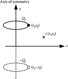
Ring charge of uniform charge density along with its image.
16.4.5 Arbitrary Line Segment Charge

Arbitrary line segment charge along with its image.16.4.6 Arbitrary Ring Segment Charge
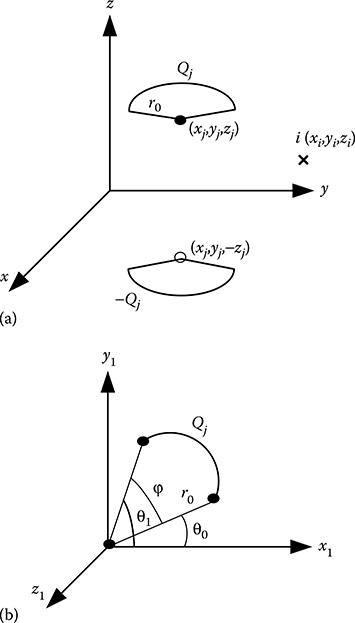
Arbitrary ring segment charge configuration for a 3D field computation: (a) ring segment charge along with its image and (b) ring segment charge after coordinate transformation.16.5 CSM with Complex Fictitious Charges

Application of CSM with complex fictitious charge for AC field calculation.
16.6 Capacitive-Resistive Field Computation by CSM
16.6.1 Capacitive-Resistive Field Computation Including Volume Resistance

Multi-dielectric arrangement with volume resistivities.

Determination of surface current density due to volume resistivities.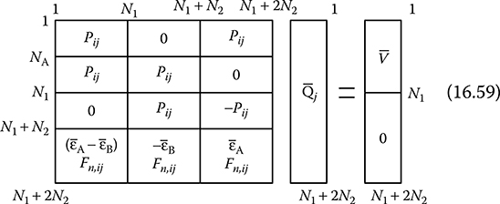
16.6.2 Capacitive-Resistive Field Computation Including Surface Resistance

Multi-dielectric arrangement with surface resistivity.
Determination of surface current density due to surface resistivity.
16.7 Field Computation by CSM under Transient Voltage
16.7.1 Transient Field Computation Including Volume Resistance

16.7.2 Transient Field Computation Including Surface Resistance

16.8 Accuracy Criteria
16.8.1 Factors Affecting Simulation Accuracy

Definition of assignment factor.16.8.2 Solution of System of Equations in CSM
16.9 Other Development in CSM
16.9.1 Least Square Error CSM

Fictitious charges and contour points for LSECSM.16.9.2 Optimized CSM
16.9.3 Region-Oriented CSM
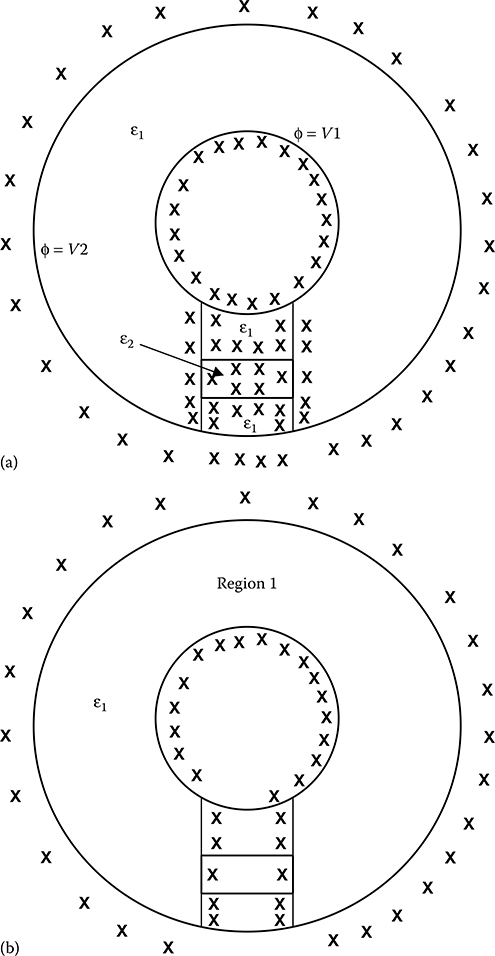
Concept of arrangement of charges in region-oriented CSM (ROCSM): (a) complete charge arrangement for ROCSM; (b) charge placement for Region 1; (c) charge placement for Region 2; (d) charge placement for Region 3 and (e) charge placement for Region 4.

16.10 Comparison of CSM with FEM
16.11 Hybrid Method Involving CSM and FEM
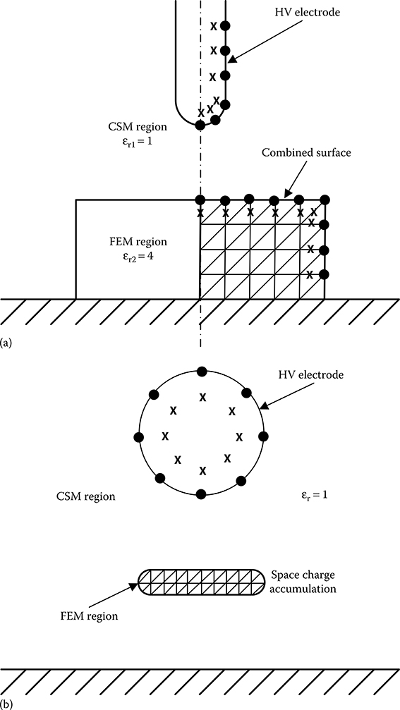
Separation of the field region into CSM region and FEM region in hybrid method: (a) application in a two-dielectric media and (b) application in space-charge modified field.16.12 CSM Examples
16.12.1 Three-Core Belted Cable

(See colour insert.) Simulation of a three-core belted cable by CSM using complex fictitious charges.16.12.2 Sphere Gap
16.12.3 Single-Core Cable Termination with Stress Cone
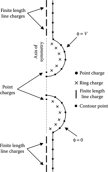
Simulation of a sphere-gap arrangement by CSM.
(See colour insert.) Simulation of fluid-filled outdoor cable termination by conventional CSM.16.12.4 Post-Type Insulator

Simulation of a post-type insulator by conventional CSM.16.12.5 Asymmetric Sphere Gaps

(See colour insert.) Simulation of an asymmetric sphere-gap arrangement by CSM.Objective Type Questions
Answers:
Bibliography