
12
Graphical Field Plotting
ABSTRACT For a clear understanding of the concept of electric field, some method for describing it, both qualitatively and quantitatively, is needed. Graphical field plotting is one such method that is dynamic in nature and illustrates the vector nature of the electric field. Graphical field maps are commonly drawn for practical configurations, which may be considered as two-dimensional or which are axi-symmetric in nature. Typically, in graphical field plotting, electric fieldlines are drawn to provide information about the field. The strength of the field is indicated by the density of the field lines. A high density of electric fieldlines indicates a strong field and vice versa. Complementary information can also be conveyed by simultaneously drawing the equipotential lines. Field maps could also be used for obtaining approximate values of system parameters such as capacitance.
Most of the practical problems have such complicated geometry that no exact method of finding the electric field is possible or feasible and approximate techniques are the only ones that can be used. Out of the several approximate techniques, numerical techniques are now extensively used to determine electric field distribution with high accuracy. Numerical techniques, which are widely used, will be discussed in detail in chapters 13 through 18. In this chapter, experimental and graphical field mapping methods are discussed. Experimental field mapping involve special equipments such as an electrolytic tank, a device for fluid flow, a conducting paper and an associated measuring system. The other mapping method is a graphical one and needs only paper and pencil. In both these methods, the exact value of the field quantities could not be determined, but accuracy level which is sufficient for practical engineering applications could be achieved. Graphical field plotting is economical compared to experimental method and is also capable of providing good accuracy when used with skill. Accuracy of the order of 5%–10% in capacitance determination could be achieved even by a non-expert simply by following the rules.
Experimental method of field mapping is based on the analogy of stationary current field with static electric field, as presented in Table 12.1, rather than directly on measurement of electric field. If the medium between electrodes is isotropic, then volume conductivity and dielectric constant do not vary with position. Then current density (J) in the stationary current field and electric field intensity (E) and electric flux density (D) in the static electric field will be in the same direction. In other words, current density and electric fieldlines are the same. Thus, for a given electrode system, if a slightly conducting material, for example, a conducting paper or an electrolyte is placed instead of a dielectric material between the electrodes, then electric fieldlines and equipotential lines will remain the same. It is well known that if one travels along a line through an electric field and measures electric scalar potential V as one goes, then the negative of the rate of change of V is equal to the component of electric field intensity E in the direction of travel. In other words, If −(∂V/∂l) is maximum, then it gives the value of E itself. If electric potential does not change with position, then the path of travel is at right angles to the electric field and is along an equipotential. Thus, electric field could be mapped by a voltmeter that will measure potential difference and two metal rods acting as probes. The probes are connected to the terminals of the voltmeter and are placed in various positions in an electric field to monitor the potential differences between the positions of the two probes. For the determination of equipotential lines one probe is kept still, while the other probe is moved. In whichever position of the moving probe the voltmeter registers a zero reading; the potential of the moving probe is same as that of the standstill probe. By marking each such position, equipotentials could be traced. TABLE 12.1 Static Electric Field Stationary Current Field Electric flux Electric current Dielectric constant Volume conductivity
For tracing electric fieldlines the two probes are kept at a constant separation distance and one probe is rotated around the other. The position of the rotating probe where the voltmeter registers a maximum reading, the electric field is changing at its maximum rate. Hence, the electric field at that location of the rotating probe is parallel to the line joining the two probes. By repeating this measurement process at several positions, the electric field could be mapped. Because a real-life voltmeter draws a current, however small it may be, the measurement of the potential differences using voltmeter could not be done with vacuum or air as the medium. In practice, measurement is carried out for the electric field that is set up in a medium, which is slightly conducting. Commonly slightly conducting paper, for example, a paper impregnated with carbon, is used. Because the paper is slightly conducting, the electric field due to the charged electrodes is almost the same as the one that would be produced in air or vacuum with similar geometry. At the same time, the paper is sufficiently conducting to supply the small current needed by the voltmeter. Alternately, electrolytic tank setup is used, which consists of a specially fabricated insulating tray. A large sheet of laminated graph paper is pasted on the base plate of the tray. The tray is then half-filled with an electrolyte and the height of the electrolyte is kept same throughout the tray. Metallic electrodes are placed in the electrolytic tank, which are shaped to conform to the boundaries of the problem, and appropriate potential difference between the electrodes is maintained.
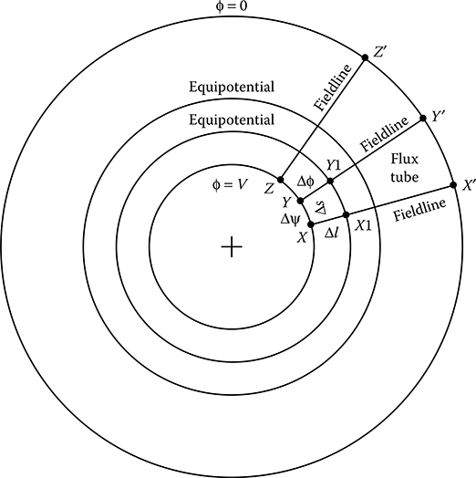
Field mapping by curvilinear squares is a graphical method based on the orthogonal property of a pair of conjugate harmonic functions and also on the geometric considerations. This method is suitable for mapping only those fields in which there is no variation of field in the direction normal to the plane of the sketch, that is, the field is two dimensional in nature. Many practical electric field problems may be considered as two dimensional, for example, the co-axial cylindrical system or a pair of long parallel wires. In these cases, the field remains same in all cross-sectional planes. It is a fact that no real system is infinitely long, but the idealization is a useful one for electric field analysis and visualization. In this method, the field region of interest is discretized into a network of curvilinear squares formed by flux or fieldlines and equipotentials. Curvilinear square is a planar geometric figure that is different from a true square, as its sides are slightly curved and slightly unequal, but which approaches a true square as its dimensions become small. A typical curvilinear square is shown in Figure 12.1. The field map thus obtained is unique for a given problem and helps in understanding the behaviour of electric field through visualization. The method of curvilinear square is capable of handling problems with complicated boundaries. A curvilinear field map is also independent of field property coefficients and could be directly applied from one physical field to another if an analogy exists between the concerned fields. FIGURE 12.1 Theoretically, curvilinear field mapping is based on Cauchy–Riemann relations, which ensures that Laplace’s equation is satisfied by a conjugate pair of harmonic functions in any orthogonal coordinate system. Hence, this method utilizes the fieldline coordinate representation of the electric field such that the electric field is always tangent to the fieldlines and depends only on the distribution of fieldlines and equipotentials. Construction of field map using curvilinear squares is based on some significant features of the electric field as described below: A conductor boundary is one of the equipotentials. Equipotential and electric field intensity (or electric flux density) are normal to each other. As a conductor boundary is an equipotential, the electric field intensity and electric flux density vectors are always perpendicular to the conductor boundaries. Electric flux lines (often termed as streamlines) originate and terminate on charges. Hence, in the case of a homogeneous and chargefree dielectric medium, electric flux lines originate and terminate on conductor boundaries. Figure 12.2 shows two co-axial cylindrical conductor boundaries having a specified potential difference (V) and extending 1 m into the plane of the paper. A fieldline is considered to leave the boundary with more positive electric potential making an angle of 90° with the boundary at the point X. If the line is extended following the rule that it is always perpendicular to the equipotentials and if the dielectric medium is considered to be homogeneous and charge free, then the fieldline will terminate normally on the boundary of the less positive conductor at the point X′, as shown in Figure 12.2. In a similar manner, another fieldline could be drawn in such a way that it starts from the point Y on the more positive conductor boundary and terminates on the point Y′ on the less positive conductor boundary. As the fieldlines are drawn perpendicular to the equipotentials everywhere, electric field intensity and electric flux density will be tangent to a fieldline everywhere on it. Consequently, no electric flux can cross any fieldline thus drawn. Therefore, if there is a charge of ΔQ on the surface of the conductor between the points X and Y, then a flux of Δψ = ΔQ will originate in this region and must terminate on the surface of the other conductor boundary between the points X′ and Y′. Such a pair of fieldlines is known as a flux tube as it seems to carry flux from one conductor to the other without losing any flux in between the two conductors. For the simplification of the interpretation of the field map, another flux tube YZ may be drawn in such a way that the same amount of flux is carried in the flux tubes XY and YZ. The method of determination of dimensions of the curvilinear square for drawing such flux tubes is described in the next section. FIGURE 12.2 Considering the length of the line joining the points X and Y to be Δs, the flux in the tube XY to be Δψ and the depth of the tube to be 1 m into the paper, the electric flux density at the midpoint of this line is then given by Therefore, considering the permittivity of dielectric medium to be ε, the electric field intensity at the midpoint of the line XY is then given by Alternately, electric field intensity could also be determined from the potential difference between the points X and X1 lying on the same fieldline on two equipotentials, as shown in Figure 12.2. Considering the length of the line joining the points X and X1 to be Δl and the potential difference between the two consecutive equipotentials to be Δϕ, the electric field intensity at the midpoint of the line X-X1 is then given by Considering Δs and Δl to be small, the two values of electric field intensity, as given by Equations 12.3 and 12.4, may be taken to be equal. Hence, For sketching the field map, consider the following: (1) homogeneous dielectric having a constant permittivity ε; (2) constant amount of electric flux per tube, that is, Δψ is constant and (3) constant potential difference between two consecutive equipotentials, that is, Δϕ is constant. Then from Equation 12.5, Δl/Δs = constant. In other words, the ratio of the distance between fieldlines as measured along an equipotential and the distance between equipotentials as measured along a fieldline must be maintained constant and not the individual lengths. The simplest ratio of lengths that can be maintained is unity, so that Δl = Δs. Then the field region is divided into curvilinear squares by the fieldlines and equipotentials. The field map thus obtained is composed of curvilinear squares of the same kind such that each square has the same potential difference across it and also has the same amount of flux through it. For a given Δϕ and Δψ, the sides of a curvilinear square are thus inversely proportional to electric field intensity. For a non-uniform field, electric field intensity varies with location and hence Δl and Δs vary with the strength of electric field. In the region of higher field strength, Δl and Δs are to be kept small, that is, the squares are to be made smaller in size where the magnitude of the field intensity is high. On the other hand, the squares are made larger in size in the field region where the field intensity is low. It may be recalled that the product of electric charge and electric potential difference is the energy of electric field. Moreover, electric charge and electric flux has a one to one correspondence. Thus, for a field map, if Δϕ and Δψ are kept constant, then their product remains constant and hence, the energy of the electric field remains constant. Therefore, curvilinear squares having the same ratio, as given by Equation 12.5, have the same energy stored in electric field regardless of the size of the square. A curvilinear square can thus be scaled up or down keeping the energy stored in the curvilinear square unaltered as long as the ratio given by Equation 12.5 remains unaltered. The fieldlines and equipotentials are typically drawn on the original sketch, which shows the conductor boundaries. Arbitrarily, one fieldline is begun from a point on the surface of the more positive conductor with a suitable value of Δl and an equipotential is drawn perpendicular to the fieldline with a value of Δs = Δl. Then another fieldline is added to complete the curvilinear square. The field map is then gradually extended throughout the field region of interest. As the field map is extended, the condition of orthogonality of fieldline and equipotential should be kept paramount, even if this results in some squares with ratios other than unity. Construction of a satisfactory field map using curvilinear squares is a trial-and-error process that involves continuous adjustment and refinement. Typically, field maps are started as a coarse map having large curvilinear squares. Then the field map is fine-tuned through successive subdivisions to form a dense field map having higher accuracy. In the process of subdivision, the lengths between consecutive fieldlines as well as equipotentials are kept equal. Before starting the construction of a field map, it is a judicious practice to examine the geometry of the system and take advantage of any symmetry that may exist in the system under consideration. This is because of the fact the lines of symmetry serve as boundaries with no flux crossing and thereby separate regions of similar field maps. Once the field map is drawn, it is possible to determine the capacitance per unit length between the two conductors using the field map. It is well known that capacitance between two conductors having a potential difference of V is given by C = Q/V, where Q is the charge on the conductor. Applying Gauss’s law on a Gaussian surface enclosing the conductor having more positive potential, Q = ψ, where ψ is the flux coming out of the conductor. Thus, C = ψ/V. FIGURE 12.3 To calculate the capacitance with the help of curvilinear rectangle, consider first an isolated curvilinear rectangle, as shown in Figure 12.3. Let the flux through it be Δψ and the potential difference across it be Δϕ. Considering the curvilinear rectangle to be small, the flux density may be assumed uniform within the curvilinear rectangle, so that where the depth is taken to be 1 m into the plane of the field map. Electric field intensity (E) and the potential difference (Δϕ) are related as Combining Equations 12.6 and 12.7 Therefore, the capacitance of the small curvilinear rectangle, which may be taken as a small field cell, is given by The total amount of flux (ψ) emanating from one conductor and terminating on the other conductor may be obtained by adding all the small amounts of flux (Δψ) through each flux tube, so that where: Δψ is assumed to be same for each flux tube Nψ is the number of flux tubes in parallel, that is, the number of curvilinear rectangles in parallel The total potential difference between the two conductors (V) may be obtained by adding all the small amounts of potential differences (Δϕ) between consecutive equipotentials starting from one conductor and finishing at the other conductor, that is, where: Δϕ is assumed to be same between any two consecutive equipotentials Nϕ is the number of equipotentials (including the two conductors) minus one, that is, the number of curvilinear rectangles in series between the two conductors Thus, capacitance per unit length of the two conductors is given by where Δs = Δl, considering the ratio of the lengths to be unity, that is, considering curvilinear squares. Hence, the determination of capacitance from the field map involves counting of curvilinear squares in two directions, one in series between the two conductors and the other in parallel around either conductor.
From Equation 12.5, it may be seen that for the same value of electric flux per tube and same potential difference between two consecutive equipotentials, Thus, in the case of a two-dielectric configuration, as shown in Figure 12.4, the ratio of the sides of curvilinear element is to be made proportional to the relative permittivity of the dielectric medium in which the field map is drawn. In other words, curvilinear rectangles are to be used. FIGURE 12.4 Moreover, the deviation of the fieldlines takes place at the boundary between the two dielectric media, as shown in Figure 12.4, which is given for charge-free dielectric media by For two-dimensional configurations comprising multi-dielectric media, the field map is first drawn in the field region where there is only one dielectric media. Then the directions of the fieldlines are changed at the boundary between the two dielectric media according to Equation 12.13. Subsequently, the ratio of the sides of the curvilinear rectangles is changed as per Equation 12.12 and the field map is extended into the field region comprising a different dielectric medium. In this way, the field map could be obtained in configurations comprising several dielectric media.
Consider a curvilinear rectangle in an axi-symmetric configuration, as shown in Figure 12.5. Let the radial distance of the centroid of the curvilinear rectangle from the axis of rotational symmetry be r. FIGURE 12.5 Considering the flux through the rectangle to be Δψ and assuming the square to be small, the electric flux density can be taken to be uniform within the rectangle and is given by Alternately, the electric field intensity as obtained from the potential difference between two consecutive equipotentials, which are the two sides of the rectangle perpendicular to the fieldlines, is given by Considering a small curvilinear rectangle, these two values of the electric field intensity could be taken as same such that Considering (1) homogeneous dielectric having a constant permittivity ε; (2) constant amount of electric flux per tube, that is, Δψ is constant and (3) constant potential difference between two consecutive equipotentials, that is, Δϕ is constant, Hence, to draw field maps in axi-symmetric configurations comprising a homogeneous dielectric, the ratio of the sides of the curvilinear rectangles is to be increased in direct proportion to the radial distance of the square from the axis of rotational symmetry. For axi-symmetric configurations comprising multiple dielectric media, Equation 12.16 is to be rewritten in the light of Equation 12.15 as Therefore, for multi-dielectric media in axi-symmetric configurations, the ratio of the sides of the curvilinear rectangles is to be increased not only in direct proportion to the radial distance of the square from the axis of rotational symmetry but also in direct proportion to the relative permittivity of the dielectric medium in which the field map is drawn. The directions of the fieldlines at the boundary between the two dielectric media are to be changed according to Equation 12.13.
1. Experimental method of field mapping is carried out using a. Highly conducting paper b. Slightly conducting paper c. Non-conducting paper d. None of the above 2. Graphical method of field mapping using curvilinear squares or rectangles is suitable for a. Two-dimensional and three-dimensional systems b. Two-dimensional and axi-symmetric systems c. Only two-dimensional system d. Only axi-symmetric system 3. Which one of the following is most commonly used for graphical field mapping in a two-dimensional system with homogeneous dielectric medium? a. Rectilinear square b. Rectilinear rectangle c. Curvilinear square d. Curvilinear rectangle 4. For field mapping in a two-dimensional system with homogeneous dielectric medium, the ratio of the distance between fieldlines as measured along an equipotential and the distance between equipotentials as measured along a fieldline is to be a. Kept constant b. Made proportional to dielectric constant of the medium c. Made inversely proportional to the dielectric constant of the medium d. Chosen arbitrarily 5. For field mapping in a two-dimensional system with multiple dielectric media, the ratio of the distance between fieldlines as measured along an equipotential and the distance between equipotentials as measured along a fieldline is to be a. Kept constant b. Made proportional to dielectric constant of the medium c. Made inversely proportional to the dielectric constant of the medium d. Chosen arbitrarily 6. For field mapping in an axi-symmetric system with homogeneous dielectric medium, the ratio of the distance between fieldlines as measured along an equipotential and the distance between equipotentials as measured along a fieldline is to be a. Kept constant b. Made proportional to dielectric constant of the medium c. Made inversely proportional to the dielectric constant of the medium d. Made proportional to the radial distance from the axis of symmetry 7. For field mapping in an axi-symmetric system with multiple dielectric media, the ratio of the distance between fieldlines as measured along an equipotential and the distance between equipotentials as measured along a fieldline is to be a. Kept constant b. Made proportional to dielectric constant of the medium c. Made proportional to the radial distance from the axis of symmetry d. Made proportional to the product of dielectric constant of the medium and the radial distance from the axis of symmetry 8. Accuracy that could be achieved in capacitance determination by graphical field plotting is typically of the order of a. 0.5%–1% b. 1%–2% c. 5%–10% d. 10%–20% 9. Which one of the following is most commonly used for graphical field mapping in a two-dimensional system with multiple dielectric media? a. Rectilinear square b. Rectilinear rectangle c. Curvilinear square d. Curvilinear rectangle 10. Determination of capacitance from the field map involves counting of curvilinear squares or rectangles a. In series between the two conductors only b. In parallel around either conductor only c. In series between the two conductors and also in parallel around either conductor d. None of the above 1) b; 2) b; 3) c; 4) a; 5) b; 6) d; 7) d; 8) c; 9) d; 10) c12.1 Introduction
12.2 Experimental Field Mapping
Analogy between Static Electric Field and Stationary Current Field
12.3 Field Mapping Using Curvilinear Squares

A typical curvilinear square.12.3.1 Foundations of Field Mapping
Field map between two co-axial cylinders.12.3.2 Sketching of Curvilinear Squares
12.3.3 Construction of Curvilinear Square Field Map
12.3.4 Capacitance Calculation from Field Map

An isolated curvilinear rectangle.
12.4 Field Mapping in Multi-Dielectric Media

Mapping in a two-dimensional configuration with multi-dielectric media.12.5 Field Mapping in Axi-Symmetric Configuration

Field mapping in an axi-symmetric configuration.Objective Type Questions
Answers:
Bibliography
1. E. Weber, ‘Mapping of fields’, Electrical Engineering, Dec, pp. 1563–1570, 1934.
2. H. Poritsky, ‘Graphical field plotting methods in engineering’, AIEE Transactions, Vol. 57, pp. 727–732, 1938.
3. R.J.W. Koopman, ‘Mapping of electric fields into curvilinear squares’, Transactions of Kansas Academy of Science, Vol. 41, pp. 233–236, 1938.
4. E.O. Willoughby, ‘Some applications of field plotting’, Journal of the Institution of Electrical Engineers—Part III: Radio and Communication Engineering, Vol. 93, No. 24, pp. 275–293, 1946.
5. K.F. Sander and J.G. Yates, ‘The accurate mapping of electric fields in an electrolytic tank’, Proceedings of the IEE—Part II: Power Engineering, Vol. 100, No. 74, pp. 167–175, 1953.
6. H. Diggle and E.R. Hartill, ‘Some applications of the electrolytic tank to engineering design problems’, Proceedings of the IEE—Part II: Power Engineering, Vol. 101, No. 82, pp. 349–364, 1954.
7. L. Tasny-Tschiassny, ‘The approximate solution of electric-field problems with the aid of curvilinear nets’, Proceedings of the IEE—Part C: Monographs, Vol. 104, No. 5, pp. 116–129, 1957.
8. J.D. Horgan and J.A. Pesavento, ‘The accurate determination of capacitance’, Electrical Engineering, Vol. 77, No. 6, p. 513, 1958.
9. S.Y. King, ‘The electric field near bundle conductors’, Proceedings of the IEE— Part C: Monographs, Vol. 106, No. 10, pp. 200–206, 1959.
10. M.M. Sakr and B. Salvage, ‘Electric stresses at conducting surfaces located in the field between plane parallel electrodes: Experiments with an electrolytic tank’, Proceedings of the Institution of Electrical Engineers, Vol. 111, No. 6, pp. 1179–1181, 1964.
11. E.S. Ip, ‘Electrostatic fields of transformer-bushing insulators’, Proceedings of the Institution of Electrical Engineers, Vol. 114, No. 11, pp. 1729–1733, 1967.
12. R.B. Goldner, ‘Rules for field plotting in a class of two-dimensional inhomogeneous conductors’, Proceedings of IEEE, Vol. 56, No. 8, pp. 1367–1368, 1968.
13. S. Ramo, J.R. Whinnery and T. van Duzer, Fields and Waves in Communication Electronics, 3rd ed., John Wiley & Sons, New York, 1994.
14. M.N.O. Sadiku, Elements of Electromagnetics, 5th ed., Oxford University Press, New York, Oxford 2009.
15. S. Tou, Visualization of Fields and Applications in Engineering, John Wiley & Sons, Chichester, UK, 2011.