15. Numerical Computation of High-Voltage Field by Finite Element Method

Search in book...
Toggle Font Controls
Create new playlist

Name your new playlist

Playlist description (optional)
Sign In

Email address

Password

Forgot Password?

or

Continue with Facebook

Continue with Google
Sign Up

Full Name

Email address

Confirm Email Address

Password

or

Continue with Facebook

Continue with Google

ABSTRACT Finite element method (FEM) is a general procedure that may be adapted to approximate the solution to various partial differential equations. Two such equations in electric field analysis are Laplace’s and Poisson’s equations. Over the course of last five decades, FEM has been proved to be very efficient in electric field analysis in two-dimensional (2D), axi-symmetric and three-dimensional (3D) systems having multiple dielectric media. Basic FEM formulations in all these systems have been discussed in this chapter. The variational approach of minimizing the functional, namely, potential energy of electric field, has been taken as the basis of FEM formulation. Details of finite elements that are mostly used in 2D and 3D systems have been presented. The chapter also highlights the procedural steps in FEM along with the nuances of its implementations such as system of FEM equations and its solution, refinement and acceptability of FEM mesh and sources of error in FEM. Use of FEM in design cycle has been also discussed from a practical viewpoint.

15.1 Introduction

Finite element method (FEM) is a numerical analysis technique to obtain solutions to the differential equations that describe, or approximately describe, a wide variety of physical problems ranging from solid, fluid and soil mechanics, to electromagnetism or dynamics. The underlying premise of the FEM is that a complicated region of interest can be subdivided into a series of smaller sub-regions in which the differential equations are approximately solved. By assembling the set of equations for each sub-region, the behaviour over the entire region of interest is determined.

It is difficult to state the exact origin of the FEM, because the basic concepts have evolved over a period of 100 or more years. The term finite element was first coined by Clough in 1960. In the early 1960s, FEM was used for approximate solution of problems in stress analysis, fluid flow, heat transfer and some other areas. In the late 1960s and early 1970s, the application of FEM was extended to a much wider variety of engineering problems. Significant advances in mathematical treatments, including the development of new elements, and convergence studies were made in 1970s. Most of the commercial FEM software packages originated in the 1970s and 1980s. FEM is one of the most important developments in computational methods to occur in the twentieth century. The method has evolved from one with applications in structural engineering at the beginning to a widely utilized and richly varied computational approach for many scientific and technological areas at present.

15.2 Basics of FEM

Images

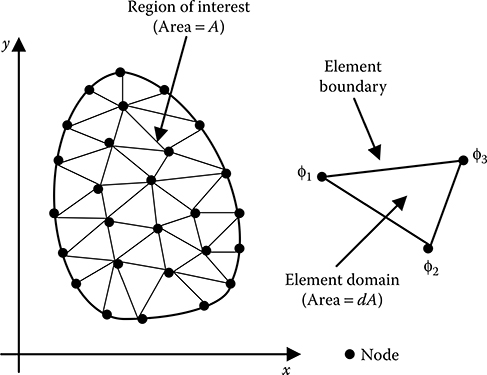
FIGURE 15.1
Depiction of region of interest, element and nodes for FEM formulation.

Using the FEM, the region of interest is discretized into smaller sub-regions called elements, as shown in Figure 15.1, and the solution is determined in terms of discrete values of some primary field variables, for example, electric potential, at the nodes. The governing equation, for example, Laplace’s or Poisson’s equations, is now applied to the domain of a single element. At the element level, the solution to the governing equation is replaced by a continuous function approximating the distribution of the field variable ϕ over the element domain, expressed in terms of the unknown nodal values ϕ₁, ϕ₂ and ϕ₃ of the solution ϕ. A system of equations in terms of ϕ₁, ϕ₂ and ϕ₃ can then be formulated for the element. Once the element equations have been determined, the elements are assembled to form the entire region of interest. Assembly is accomplished using the basic rule that the value of the field variable at a node must be the same for each element that shares that node. The solution ϕ to the problem becomes a piecewise approximation, expressed in terms of the nodal values of ϕ. The assembly procedure results in a system of linear algebraic equations.

Several approaches can be used to transform the physical formulation of the problem to its finite element discrete analogue. If the physical formulation of the problem is known as a differential equation, for example, Laplace’s or Poisson’s equations, then the most popular method of its finite element formulation is the Galerkin method. If the physical problem can be formulated as minimization of a functional, then the variational formulation of the finite element equations is usually used. For problems in high-voltage fields, the functional turns out to be the energy stored in the electric field.

A third and even more versatile approach to derive element properties is known as the weighted residuals approach. The weighted residuals approach begins with the governing equations of the problem and proceeds without relying on a variational statement. This approach is advantageous because it makes it possible to extend the FEM to problems where no functional is available.

15.3 Procedural Steps in FEM

In general terms, the main steps of the finite element solution procedure are as follows.

At the beginning the region of interest is discretized into finite elements.
Suitable functions are considered to interpolate the field variables over the element.
The matrix equation for the finite element is formed relating the nodal values of the unknown field variables to other physical parameters.
Global equation system is formed for the entire region of interest by assembling all the element equations. Element connectivities are used for the assembly process. Boundary conditions, which are not accounted in element equations, are imposed before the solution of equations.
The finite element global equation system is solved to get the nodal values of the sought field variables.
In many cases, additional parameters need to be calculated after the solution of global equation system. For example, in high-voltage field problems, electric field intensity, electric flux density and charges are of interest in addition to electric potential, which are obtained after solution of the global equation system.

15.4 Variational Approach towards FEM Formulation

For high-voltage field problems, the principle of minimum potential energy is used in this approach. The principle of minimum potential energy can be stated as: Out of all possible potential functions, ϕ(x,y,z), the one which minimizes the total potential energy is the potential solution that will satisfy equilibrium, and will be the actual potential due to the applied field forces.

Thus, a potential function that will minimize the functional, that is, potential energy, is desired. Minimization of functionals falls within the field of variational calculus. In most cases, an exact function is impossible to determine, necessitating the use of approximate numerical methods. Minimization of potential energy in a finite element formulation is carried out using the energy approach. FEM develops the equations from simple element shapes, in which the unknowns of the solution are the potentials at the nodes. The calculus of variations enables the energy equation to be reduced to a set of simultaneous equations with the nodal potentials as the unknown quantities.

15.4.1 FEM Formulation in a 2D System with Single-Dielectric Medium

The potential energy in a two-dimensional (2D) electric field is given by

$U_{t o t a 1} = \iint_{A} \frac{1}{2} ε_{0} ε_{r} | \vec{E} |^{2} \cdot l \cdot d A (15.1)$

$or, U_{t o t a 1} = \iint_{A} \frac{1}{2} ε_{0} ε_{r} | - \vec{∇} ϕ |^{2} \cdot l \cdot d A (15.2)$

where:

E = electric field intensity
ϕ = electric potential
l = length normal to the area A (usually considered as unity for 2D field)
ε₀ = permittivity of free space
ε_r = relative permittivity of dielectric

The integration of Equation 15.1 must be carried out over the area A, which is identical to the field region under consideration, as shown in Figure 15.1. Because this area must be finite, FEM cannot be applied to the problems with open fields without modifications.

To apply FEM, the region of interest is to be discretized by so-called finite elements, as shown in Figure 15.1. If a region of interest is divided into elements such that the continuity of electric potential between elements is enforced, then the total potential energy is equal to the sum of the individual energies of each element. For N number of elements, the total potential energy can then be stated as follows:

$U_{t o t a 1} = Σ_{e = 1}^{N} U (e) (15.3)$

To minimize the total potential energy, U, of the entire region of interest, U(e) must be minimized for each element. Seeking a set of nodal potentials for each element will minimize U(e). Observe that the functional U(e) is a function only of the nodal potentials. Using calculus of variations, an extremization of U(e) occurs when the vector of the first partial derivatives with respect to ϕ is zero.

The simplest 2D element is the linear triangular element, as shown in Figure 15.2. For this element, there are three nodes at the vertices of the triangle, which are numbered around the element in the anti-clockwise direction. Electric potential ϕ is assumed to be varying linearly within the element such that

$ϕ = α_{1} + α_{2} x + α_{3} y (15.4)$

Hence,

$\begin{matrix} \begin{matrix} E_{x} = - \frac{\partial ϕ}{\partial x} = - α_{2} & and \end{matrix} & E_{y} = - \frac{\partial ϕ}{\partial y} = - α_{3} \end{matrix} (15.5)$

Thus, for this element, the electric field intensity components are constant throughout the element. As a result, this type of element is also known constant stress element (CST).

Now, considering a triangular element, as shown in Figure 15.2

Images

FIGURE 15.2
Linear triangular element.

$\begin{matrix} ϕ_{1} = α_{1} + α_{2} x_{1} + α_{3} y_{1} \\ ϕ_{2} = α_{1} + α_{2} x_{2} + α_{3} y_{2} \\ ϕ_{3} = α_{1} + α_{2} x_{3} + α_{3} y_{3} \end{matrix} (15.6)$

Therefore, from Equation 15.6

$\begin{matrix} α_{2} = \frac{| \begin{matrix} 1 & ϕ_{1} & y_{1} \\ 1 & ϕ_{2} & y_{2} \\ 1 & ϕ_{3} & y_{3} \end{matrix} |}{| \begin{matrix} 1 & x_{1} & y_{1} \\ 1 & x_{2} & y_{2} \\ 1 & x_{3} & y_{3} \end{matrix} |} \\ or, α_{2} = \frac{1}{D} [ϕ_{1} (y_{2} - y_{3}) + ϕ_{2} (y_{3} - y_{1}) + ϕ_{3} (y_{1} - y_{2})] \end{matrix} (15.7)$

Where:

$\begin{matrix} D = & (x_{2} y_{3} - x_{3} y_{2}) + (x_{3} y_{1} - x_{1} y_{3}) + (x_{1} y_{2} - x_{2} y_{1}) \\ = & 2 times the area of the triangle \end{matrix} (15.8)$

Similarly,

$α_{3} = \frac{1}{D} [ϕ_{1} (x_{3} - x_{2}) + ϕ_{2} (x_{1} - x_{3}) + ϕ_{3} (x_{2} - x_{1})] (15.9)$

The magnitude of the electric field intensity within an element T,

$| {\vec{E}}_{T} | = \sqrt{| E_{x}^{2} | + | E_{y}^{2} |} = \sqrt{α_{2}^{2} + α_{3}^{2}} (15.10)$

Hence, the electric potential energy in an element T

$U_{T} = \frac{1}{2} ε_{0} ε_{r} | {\vec{E}}_{T} |^{2} A \cdot l = \frac{1}{2} ε_{0} ε_{r} A \cdot l \cdot (α_{2}^{2} + α_{3}^{2}) (15.11)$

For electric potential energy in an element to be minimum,

$\frac{\partial U_{T}}{\partial ϕ_{1}} = \frac{1}{2} ε_{0} ε_{r} A \cdot l \cdot 2 (α_{2} \frac{\partial α_{2}}{\partial ϕ_{1}} + α_{3} \frac{\partial α_{3}}{\partial ϕ_{1}}) = 0 (15.12)$

Equation 15.12 is to be applied to every node where the unknown potential is to be determined. It may be noted here that the node under consideration may belong to more than one element. Then Equation 15.12 is to be applied for all such elements considering the node under consideration as node 1 and the other two nodes of the element being node 2 and node 3 taken in the anti-clockwise direction.

Now,

$\frac{\partial α_{2}}{\partial ϕ_{1}} = \frac{y_{2} - y_{3}}{D}, \frac{\partial α_{3}}{\partial ϕ_{1}} = \frac{x_{3} - x_{2}}{D} and A = D / 2$

Therefore, from Equation 15.12

$\begin{array}{r} \frac{1}{2} ε_{0} ε_{r} \frac{D}{2} \cdot l \cdot 2 (α_{2} \frac{y_{2} - y_{3}}{D} + α_{3} \frac{x_{3} - x_{2}}{D}) = 0 \\ or, \frac{1}{2} ε_{0} ε_{r} \cdot l \cdot [α_{2} (y_{2} - y_{3}) + α_{3} (x_{3} - x_{2})] = 0 \end{array} (15.13)$

Hence, from Equations 15.7, 15.9 and 15.13

$\begin{matrix} \frac{ε_{0} ε_{r} l}{2 D} {[ϕ_{1} (y_{2} - y_{3}) + ϕ_{2} (y_{3} - y_{1}) + ϕ_{3} (y_{1} - y_{2})] [y_{2} - y_{3}] \\ + [ϕ_{1} (x_{3} - x_{2}) + ϕ_{2} (x_{1} - x_{3}) + ϕ_{3} (x_{2} - x_{1})] [x_{3} - x_{2}]} = 0 \end{matrix} (15.14a)$

$\begin{matrix} or, \frac{ε_{r}}{D} {ϕ_{1} [(x_{3} - x_{2})^{2} + (y_{2} - y_{3})^{2}] + ϕ_{2} [(x_{3} - x_{2}) (x_{1} - x_{3}) + (y_{2} - y_{3}) (y_{3} - y_{1})] \\ + ϕ_{3} [(x_{3} - x_{2}) (x_{2} - x_{1}) + (y_{2} - y_{3}) (y_{1} - y_{2})]} = 0 \end{matrix} (15.14b)$

$or, K_{1 T} ϕ_{1} + K_{2 T} ϕ_{2} + K_{3 T} ϕ_{3} = 0 (15.15)$

where:

$\begin{array}{l} K_{1 T} = \frac{ε_{r T}}{D_{T}} [(x_{3 T} - x_{2 T})^{2} + (y_{2 T} - y_{3 T})^{2}] \\ K_{2 T} = \frac{ε_{r T}}{D_{T}} [(x_{3 T} - x_{2 T}) (x_{1 T} - x_{3 T}) + (y_{2 T} - y_{3 T}) (y_{3 T} - y_{1 T})] \\ K_{3 T} = \frac{ε_{r T}}{D_{T}} [(x_{3 T} - x_{2 T}) (x_{2 T} - x_{1 T}) + (y_{2 T} - y_{3 T}) (y_{1 T} - y_{2 T})] \end{array} (15.16)$

where:

Subscript T denotes the element number
D_T is twice the area of the element, as given by Equation 15.8
ε_rT is the permittivity of the dielectric within the element

Discretization using triangular elements is usually done is such a way that one particular node is connected to either six other nodes in hexagonal connectivity, as shown in Figure 15.3a, or to eight other nodes in octagonal connectivity, as shown in Figure 15.3b. For hexagonal connectivity, an equation may be formed involving potentials of all the six nodes surrounding the node ‘0’ applying Equation 15.15. In such case, for every element, node 0 of Figure 15.3 is considered to be node 1 of Equation 15.15 and the other two nodes are considered to be node 2 and node 3 in the anti-clockwise direction. Application of Equation 15.15 thus results in six simultaneous linear equations, the summation of which may be represented as follows.

Images

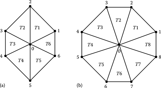
FIGURE 15.3
Nodal connectivity – (a) 6 elements (hexagonal) and (b) 8 elements (octagonal).

$F ϕ_{1} + F_{2} ϕ_{2} + F_{3} ϕ_{3} + F_{4} ϕ_{4} + F_{5} ϕ_{5} + F_{6} ϕ_{6} + F_{0} ϕ_{0} = 0 (15.17)$

where:

$\begin{array}{l} F_{1} = K_{2 (T 1)} + K_{3 (T 6)} \\ F_{2} = K_{2 (T 2)} + K_{3 (T 1)} \\ F_{3} = K_{2 (T 3)} + K_{3 (T 2)} \\ F_{4} = K_{2 (T 4)} + K_{3 (T 3)} \\ F_{5} = K_{2 (T 5)} + K_{3 (T 4)} \\ F_{6} = K_{2 (T 6)} + K_{3 (T 5)} \\ and F_{0} = Σ_{T = 1}^{6} K_{1 T} \end{array} (15.18)$

Application of Equation 15.17 to all the nodes having unknown potential will generate the FEM system of simultaneous linear equations, which needs to be solved for determining the node potentials. Equations 15.17 and 15.18 could be suitably modified for octagonal nodal connectivity. Here, it may also be noted that FEM formulation as described above automatically takes into account the unequal elemental sizes as the coefficients as in Equation 15.18 are all computed in terms of nodal coordinates that may have any numerical value.

15.4.2 FEM Formulation in 2D System with Multi-Dielectric Media

For computing electric field in multi-dielectric media, triangular elements are so positioned that any given triangular element comprises only one dielectric medium. In other words, a set of nodal points are to be placed on the interface between two dielectrics, as shown in Figure 15.4. Hence, the coefficients K_1T, K_2T and K_3T for any node are to be calculated depending on its nodal position (i.e., 1, 2 or 3) in an element considering the proper value of ε_r.

While applying Equation 15.17 for the nodal connectivity shown in Figure 15.4, the following modifications need to be made for F₂, F₅ and F₀ keeping the others unchanged.

$F_{2} = K_{2 (T 2)} + K_{3 (T 1)}, F_{5} = K_{2 (T 5)} + K_{3 (T 4)} and F_{0} = Σ_{T = 1}^{6} K_{1 T}$

where:

$\begin{matrix} K_{2 (T 2)} = \frac{ε_{r 2}}{D_{T 2}} [(x_{3} - x_{2}) (x_{0} - x_{3}) + (y_{2} - y_{3}) (y_{3} - y_{0})] \\ K_{3 (T 1)} = \frac{ε_{r 1}}{D_{T 1}} [(x_{2} - x_{1}) (x_{1} - x_{0}) + (y_{1} - y_{2}) (y_{0} - y_{1})] \\ K_{2 (T 5)} = \frac{ε_{r 1}}{D_{T 5}} [(x_{6} - x_{5}) (x_{0} - x_{6}) + (y_{5} - y_{6}) (y_{6} - y_{0})] \\ K_{3 (T 4)} = \frac{ε_{r 2}}{D_{T 4}} [(x_{5} - x_{4}) (x_{4} - x_{0}) + (y_{4} - y_{5}) (y_{0} - y_{4})] \end{matrix}$

Images

FIGURE 15.4
Elemental discretization for multi-dielectric media.

For the computation of F₀, K_1T is to be calculated considering ε_r1 for the elements 1, 5 and 6 and considering ε_r2 for the elements 2, 3 and 4, using Equation 15.16. For example, for elements T3 and T6, respectively, the expressions for K_1T will be as follows:

$\begin{matrix} K_{1 (T 3)} = \frac{ε_{r 2}}{D_{T 3}} [(x_{4} - x_{3})^{2} + (y_{3} - y_{4})^{2}] \\ and K_{1 (T 6)} = \frac{ε_{r 1}}{D_{T 6}} [(χ_{1} - x_{6})^{2} + (y_{6} - y_{1})^{2}] \end{matrix}$

Here, it may be noted that no separate formulation is required for multi-dielectric media in FEM in contrast to FDM.

15.4.3 FEM Formulation in Axi-Symmetric System

As already discussed, the electric potential energy in a triangular element is

$U_{e} = \frac{1}{2} ε_{0} ε_{r} | \vec{E} |^{2} \cdot A \cdot l (15.19)$

where:

(A·l) is the volume of the element

For an axi-symmetric system, this volume is created due to the rotation of a triangular element around the axis of symmetry (Figure 15.5). The area of the triangle being A, l should then be the mean length of rotation, that is, 2π times the radial distance of the centroid of the triangle.

Images

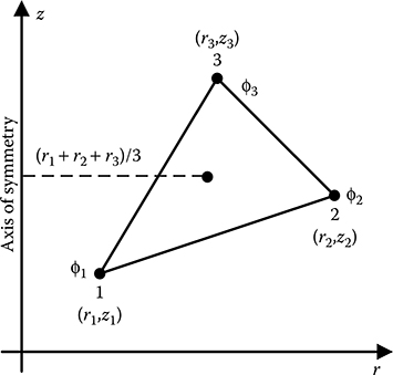
FIGURE 15.5
Triangular element for an axi-symmetric formulation.

Therefore,

$l = 2 π \frac{(r_{1} + r_{2} + r_{3})}{3} (15.20)$

Putting this expression for l in Equation 15.14b

$\begin{array}{l} \frac{ε_{0} ε_{r}}{2 D} \cdot \frac{2 π (r_{1} + r_{2} + r_{3})}{3} {ϕ_{1} [(r_{3} - r_{2})^{2} + (z_{2} - z_{3})^{2}] \\ + ϕ_{2} [(r_{3} - r_{2}) (r_{1} - r_{3}) + (z_{2} - z_{3}) (z_{3} - z_{1})] \\ + ϕ_{3} [(r_{3} - r_{2}) (r_{2} - r_{1}) + (z_{2} - z_{3}) (z_{1} - z_{2})]} = 0 \end{array} (15.21)$

Therefore, from the above equation in an axi-symmetric system,

K_1Tϕ₁ + K_2Tϕ₂ + K_3Tϕ₃ = 0

where:

$\begin{matrix} K_{1 T} = \frac{R ε_{r T}}{D_{T}} [(r_{3 T} - r_{2 T})^{2} + (z_{2 T} - z_{3 T})^{2}] \\ K_{2 T} = \frac{R ε_{r T}}{D_{T}} [(r_{3 T} - r_{2 T}) (r_{1 T} - r_{3 T}) + (z_{2 T} - z_{3 T}) (z_{3 T} - z_{1 T})] \\ K_{3 T} = \frac{R ε_{r T}}{D_{T}} [(r_{3 T} - r_{2 T}) (r_{2 T} - r_{1 T}) + (z_{2 T} - z_{3 T}) (z_{1 T} - z_{2 T})] \\ and R = (r_{1} + r_{2} + r_{3}) \end{matrix} (15.22)$

For the axi-symmetric system with multi-dielectric media, the modifications to be brought in are the same as those described for a 2D formulation discussed in Section 15.4.2.

15.4.4 Shape Function, Global and Natural Coordinates

Solution of FEM equations gives the field variables at the nodes, but the field variables at different points inside the element are also needed. For this purpose, shape functions are used to interpolate the nodal values of field variables to compute the corresponding values at arbitrary points inside the elements.

Consider that one vertex of the triangle is moved holding the other two fixed. Then both the deformed and non-deformed triangles can be drawn on top of one another, as shown in Figure 15.6a.

Assuming the deformation to be linear, the areas of the deformed triangles can be calculated from the base and height of the triangle. As the base remains constant, the area is a linear function of the height, that is, the displacement of the node within the triangle. As all the three nodes could be displaced, so three linear functions need to be written to describe the displacement of an interior point due to the displacement of each of the nodes. The displacement of the interior point will be computed by summing the displacement due to each of the three nodes of the triangle.

Images

FIGURE 15.6
(a) Triangle in non-deformed and deformed states and (b) interpolation at an interior point.

As shown in Figure 15.6b, the interior point divides the triangle into three sub-triangles. All three nodes may move and hence the motion of the interior point is some combination of their displacements. Let A1, A2 and A3 be the area of each of sub-triangles and A be the total area of the triangular element. Then A = A1 + A2 + A3.

Therefore, the shape functions are defined as follows:

$L_{1} = \frac{A 1}{A}, L_{2} = \frac{A 2}{A} and L_{3} = \frac{A 3}{A} (15.23)$

In terms of the nodal coordinates, the shape functions are given by

$\begin{matrix} L_{1} = \frac{1}{2 A} [(x_{1} y_{2} - x_{2} y_{1}) + (y_{1} - y_{2}) x + (x_{2} - x_{1}) y] \\ L_{2} = \frac{1}{2 A} [(x_{2} y_{3} - x_{3} y_{2}) + (y_{2} - y_{3}) x + (x_{3} - x_{2}) y] \\ L_{3} = \frac{1}{2 A} [(x_{3} y_{1} - x_{1} y_{3}) + (y_{3} - y_{1}) x + (x_{1} - x_{3}) y] \end{matrix} (15.24)$

$A = \frac{1}{2} [(x_{2} y_{3} - x_{3} y_{2}) + (x_{3} y_{1} - x_{1} y_{3}) + (x_{1} y_{2} - x_{2} y_{1})] = \frac{1}{2} \det | \begin{matrix} 1 & x_{1} & y_{1} \\ 1 & x_{2} & y_{2} \\ 1 & x_{3} & y_{3} \end{matrix} |$

The same shape functions can be used to compute the coordinates of a point interior to the triangle:

$\begin{matrix} x = L_{1} x_{1} + L_{2} x_{2} + L_{3} x_{3} \\ y = L_{1} y_{1} + L_{2} y_{2} + L_{3} y_{3} \end{matrix} (15.25)$

From Equation 15.25, it is obvious that the values of the shape functions for node 1 are (1,0,0), for node 2 are (0,1,0) and for node 3 are (0,0,1). The shape functions are not independent of one another because L₁ + L₂ + L₃ = 1. Hence, if two shape functions are known, then it is possible to compute the third. Introducing the natural coordinates within the triangle (ξ,η) such that

$\begin{matrix} L_{1} = ξ, L_{2} = η \\ Then \\ L_{3} = 1 - ξ - η \end{matrix} (15.26)$

The representation of natural coordinates is shown in Figure 15.7.

A local coordinate system that relies on the element geometry for its definition and whose coordinates range between zero and unity within the element is known as the natural coordinate system. Natural coordinate systems have the property that one particular coordinate has unit value at one node of the element and zero value at the other nodes. Use of natural coordinates is advantageous in deriving interpolation functions and also in the development of curved-sided elements.

Substituting ξ and η in Equation 15.25, the relationship between the global coordinates (x,y) and the natural coordinates (ξ,η) can be obtained as given below:

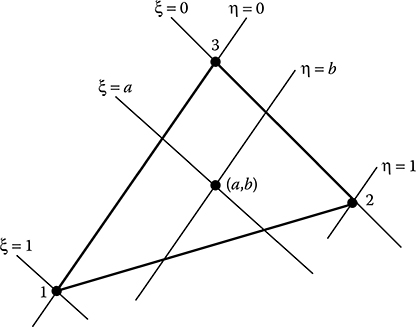
$\begin{array}{l} x = (x_{1} - x_{3}) ξ + (x_{2} - x_{3}) η + x_{3} \\ y = (y_{1} - y_{3}) ξ + (y_{2} - y_{3}) η + y_{3} \end{array} (15.27a)$

Images

FIGURE 15.7
Representation of natural coordinates.

The above equation can be used to compute the natural coordinates. If any point within the triangle is given, then the coordinates of the vertices (x₁,y₁), (x₂,y₂) and (x₃,y₃) are known along with the coordinate of the given point (x,y). Therefore, Equation 15.27 can be solved for ξ and η. Subsequently, if the field variable, say electric potential, is known at the nodes, then the natural coordinates can be used to compute the field variable for the point at (x,y). For example,

$ϕ (x, y) = (ϕ_{1} - ϕ_{3}) ξ + (ϕ_{2} - ϕ_{3}) η + ϕ_{3} (15.27b)$

15.4.5 Derivation of Field Variables Using Natural Coordinates

The potential within the element can therefore be viewed as a function of (x,y) or (ξ,η). Therefore, using the chain rule of derivatives,

${\begin{matrix} \frac{\partial ϕ}{\partial ξ} \\ \frac{\partial ϕ}{\partial η} \end{matrix}} = {\begin{matrix} \frac{\partial x}{\partial ξ} & \frac{\partial y}{\partial ξ} \\ \frac{\partial x}{\partial η} & \frac{\partial y}{\partial η} \end{matrix}} {\begin{matrix} \frac{\partial ϕ}{\partial x} \\ \frac{\partial ϕ}{\partial y} \end{matrix}} = J {\begin{matrix} \frac{\partial ϕ}{\partial x} \\ \frac{\partial ϕ}{\partial y} \end{matrix}} (15.28)$

where:

J is the Jacobian matrix of the transformation

From Equation 15.27a, the Jacobian can be obtained as

$\begin{matrix} J = [\begin{matrix} (x_{1} - x_{3}) & (y_{1} - y_{3}) \\ (x_{2} - x_{3}) & (y_{2} - y_{3}) \end{matrix}] & \begin{matrix} and & J^{- 1} = \frac{1}{2 A} [\begin{matrix} (y_{2} - y_{3}) & - (y_{1} - y_{3}) \\ - (x_{2} - x_{3}) & (x_{1} - x_{3}) \end{matrix}] \end{matrix} \end{matrix} (15.29)$

where:

$\begin{matrix} \det J = & (x_{1} - x_{3}) (y_{2} - y_{3}) - (x_{2} - x_{3}) (y_{1} - y_{3}) \\ = & 2 (area of the triangular element) \end{matrix} (15.30)$

From Equations 15.28 and 15.29,

${\begin{matrix} \frac{\partial ϕ}{\partial x} \\ \frac{\partial ϕ}{\partial y} \end{matrix}} = J^{- 1} {\begin{matrix} \frac{\partial ϕ}{\partial ξ} \\ \frac{\partial ϕ}{\partial η} \end{matrix}} = \frac{1}{2 A} [\begin{matrix} (y_{2} - y_{3}) & - (y_{1} - y_{3}) \\ - (x_{2} - x_{3}) & (x_{1} - x_{3}) \end{matrix}] {\begin{matrix} \frac{\partial ϕ}{\partial ξ} \\ \frac{\partial ϕ}{\partial η} \end{matrix}} (15.31)$

From Equations 15.27b and 15.31,

${\begin{matrix} - E_{x} \\ - E_{y} \end{matrix}} = \frac{1}{D} [\begin{matrix} (y_{2} - y_{3}) & - (y_{1} - y_{3}) \\ - (x_{2} - x_{3}) & (x_{1} - x_{3}) \end{matrix}] [\begin{matrix} (ϕ_{1} - ϕ_{3}) \\ (ϕ_{2} - ϕ_{3}) \end{matrix}] (15.32)$

where:

D = 2A

From Equation 15.32

$\begin{matrix} E_{x} = & \frac{1}{D} [(y_{1} - y_{3}) (ϕ_{2} - ϕ_{3}) - (y_{2} - y_{3}) (ϕ_{1} - ϕ_{3})] \\ = & \frac{1}{D} [ϕ_{1} (y_{3} - y_{2}) + ϕ_{2} (y_{1} - y_{3}) + ϕ_{3} (y_{2} - y_{1})] \end{matrix} (15.33a)$

$\begin{matrix} and E_{y} = & \frac{1}{D} [(χ_{2} - x_{3}) (ϕ_{1} - ϕ_{3}) - (x_{1} - x_{3}) (ϕ_{2} - ϕ_{3})] \\ = & \frac{1}{D} [ϕ_{1} (x_{2} - y_{3}) + ϕ_{2} (x_{3} - x_{1}) + ϕ_{3} (x_{1} - x_{2})] \end{matrix} (15.33b)$

Equations 15.33a and 15.33b thus give ${\vec{E}}_{x} = - α_{2}$ and ${\vec{E}}_{y} = - α_{3}$ , which are same as those obtained in Equations 15.5, 15.7 and 15.9.

PROBLEM 15.1

The nodal coordinates of a linear triangular element are (1,1), (3,2) and (2,3) mm, respectively. The potentials at the three nodes are as follows: node 1, 100 V; node 2, 150 V and node 3, 200 V. Calculate the potential and the electric field intensity components at the point P(2,2) mm within the triangular element.

Solution:

$\begin{matrix} A & = \frac{1}{2} [(x_{2} y_{3} - x_{3} y_{2}) + (x_{3} y_{1} - x_{1} y_{3}) + (x_{1} y_{2} - x_{2} y_{1})] \\ = \frac{1}{2} [(3 \times 3 - 2 \times 2) + (2 \times 1 - 1 \times 3) + (1 \times 2 - 3 \times 1)] = \frac{3}{2} \\ L_{1} & = \frac{1}{2 A} [(x_{1} y_{2} - x_{2} y_{1}) + (y_{1} - y_{2}) x + (x_{2} - x_{1}) y] \\ = \frac{1}{2 \times 3} [(1 \times 2 - 3 \times 1) + (1 - 2) 2 + (3 - 1) 2] = \frac{1}{3} \\ L_{2} & = \frac{1}{2 A} [(x_{2} y_{3} - x_{3} y_{2}) + (y_{2} - y_{3}) x + (x_{3} - x_{2}) y] \\ = \frac{2}{2 \times 3} [(3 \times 3 - 2 \times 2) + (2 - 3) 2 + (2 - 3) 2] = \frac{1}{3} \\ L_{3} & = \frac{1}{2 A} [(x_{3} y_{1} - x_{1} y_{3}) + (y_{3} - y_{1}) x + (x_{1} - x_{3}) y] \\ = \frac{2}{2 \times 3} [(2 \times 1 - 1 \times 3) + (3 - 1) 2 + (1 - 2) 2] = \frac{1}{3} \end{matrix}$

Therefore,

$\begin{array}{l} ϕ (2, 2) = \frac{1}{3} \times 100 + \frac{1}{3} \times 150 + \frac{1}{3} \times 200 = 150 V \\ α_{2} = \frac{1}{D} [ϕ_{1} (y_{2} - y_{3}) + ϕ_{2} (y_{3} - y_{1}) + ϕ_{3} (y_{1} - y_{2})] \\ = \frac{1}{2 A} [100 (2 - 3) + 150 (3 - 2) + 200 (1 - 2)] \\ = - 50 V / m m \\ α_{3} = \frac{1}{D} [ϕ_{1} (x_{3} - x_{2}) + ϕ_{2} (x_{1} - x_{3}) + ϕ_{3} (x_{2} - x_{1})] \\ = \frac{1}{2 A} [100 (2 - 3) + 150 (1 - 2) + 200 (3 - 1)] \\ = 50 V / m m \end{array}$

Hence,

${\vec{E}}_{x} (2, 2) = - α_{2} = 50 V / m m and {\vec{E}}_{y} (2, 2) = - α_{3} = - 50 V / m m$

It is to be noted here that the nodes 1(1,1), 2(3,2) and 3(2,3) are taken in the anti-clockwise direction. If these three nodes are taken in the clockwise direction, for example, nodes 1(1,1), 2(2,3) and 3(3,2), then the area of the triangle becomes negative. This is why the nodes of a triangular element have to be taken always in the anti-clockwise direction.

15.4.6 Other Types of Elements for 2D and Axi-Symmetric Systems

15.4.6.1 Quadratic Triangular Element

There are six nodes on this element, as shown in Figure 15.8. Three nodes are at the three vertices and three nodes are at the middle of the three sides of the triangle.

Electric potential is assumed to be a quadratic function of global coordinates (x,y) within the element such that

$ϕ = α_{1} + α_{2} x + α_{3} y + α_{4} x^{2} + α_{5} x y + α_{6} y^{2} (15.34)$

Thus, the electric field intensity components are as follows:

$E_{x} = - \frac{\partial ϕ}{\partial x} = - (α_{2} + 2 α_{4} x + α_{5} y) and E_{y} = - \frac{\partial ϕ}{\partial y} = - (α_{3} + 2 α_{6} y + α_{5} x) (15.35)$

Thus, the electric field intensity varies linearly within the triangular element. Hence, this type of element is known linear stress triangle, which gives better results than the CST.

Images

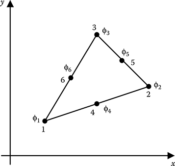
FIGURE 15.8
Quadratic triangular element.

In terms of the natural coordinates, the six shape functions for this element are as follows:

$\begin{array}{l} L_{1} = ξ (2 ξ - 1), L_{2} = η (2 η - 1), L_{3} = ζ (2 ζ - 1); \\ L_{4} = 4 ξ η, L_{5} = 4 η ζ, L_{6} = 4 ζ ξ \end{array} (15.36)$

Where:

ζ = 1 − ξ − η

Electric potential function within the element is written as

$ϕ = L_{1} ϕ_{1} + L_{2} ϕ_{2} + L_{3} ϕ_{3} + L_{4} ϕ_{4} + L_{5} ϕ_{5} + L_{6} ϕ_{6} (15.37)$

15.4.6.2 Linear Quadrilateral Element

In this element, there are four nodes at the four corners of a quadrilateral, as shown in Figure 15.9. In the natural coordinate system (ξ,η), the four shape functions are given as follows.

$\begin{array}{l} L_{1} = \frac{1}{4} (1 - ξ) (1 - η), L_{2} = \frac{1}{4} (1 + ξ) (1 - η) \\ L_{3} = \frac{1}{4} (1 + ξ) (1 + η L_{4} = \frac{1}{4} (1 - ξ) (1 + η) \end{array} (15.38)$

At any point inside the element, L₁ + L₂ + L₃ + L₄ = 0.

In a generalized way, the shape function can be written as

$L_{i} = \frac{1}{4} (1 + ξ ξ_{i}) (1 + η η_{i}), i = 1, ..., 4$

Images

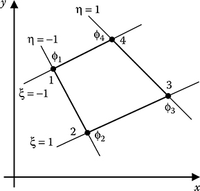
FIGURE 15.9
Linear quadrilateral element.

The electric potential within the element varies as

$ϕ = L_{1} ϕ_{1} + L_{2} ϕ_{2} + L_{3} ϕ_{3} + L_{4} ϕ_{4} (15.39)$

15.4.6.3 Quadratic Quadrilateral Element

There are eight nodes in this element, four nodes at the four corners of the quadrilateral and four nodes at the middle of the four sides, as shown in Figure 15.10.

Images

FIGURE 15.10
Quadratic quadrilateral element.

The eight shape functions can be represented in natural coordinates as follows:

$\begin{array}{l} L_{1} = \frac{1}{4} (1 - ξ) (η - 1) (ξ + η + 1 L_{2} = \frac{1}{4} (1 + ξ) (η - 1) (η - ξ + 1) \\ L_{3} = \frac{1}{4} (1 + ξ) (1 + η) (ξ + η - 1), L_{4} = \frac{1}{4} (ξ - 1) (η + 1) (ξ - η + 1) \\ L_{5} = \frac{1}{2} (1 - ξ^{2}) (1 - η), L_{6} = \frac{1}{2} (1 + ξ) (1 - η^{2}) \\ L_{7} = \frac{1}{2} (1 - ξ^{2}) (1 + η), L_{8} = \frac{1}{2} (1 - ξ) (1 - η^{2}) \end{array} (15.40)$

At any point inside the element, $Σ_{i = 1}^{8} L_{i} = 0$ .

The electric potential function within the element is given by $ϕ = Σ_{i = 1}^{8} L_{i} ϕ_{i}$ . For an axi-symmetric system, all the elements resemble a ring having its axis same as the axis of symmetry of the system, whose cross section will be as per the figures shown in the respective subsections hereabove.

PROBLEM 15.2

For the 2D configuration having a single-dielectric medium, as shown in Figure 15.11, write the FEM equations for the nodes having unknown node potentials. Consider the finite elements to be linear triangular elements.

Solution:

Images

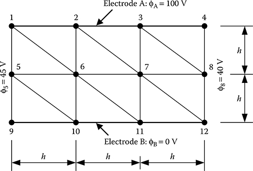
FIGURE 15.11
Pertaining to Problem 15.2.

Out of the 12 nodes shown in Figure 15.11, the potential of only two nodes are unknown, namely, nodes 6 and 7. Both these nodes belong to six elements in the mesh, as shown in Figure 15.11. Assuming the coordinate of node 9 to be (0,0) and considering h = 1, the coordinates of the other nodes are determined accordingly.

For node 6:

F₁ϕ₁ + F₂ϕ₅ + F₃ϕ₁₀ + F₄ϕ₁₁ + F₅ϕ₇ + F₆ϕ₂ + F₀ϕ₆ = 0

Where:

ϕ₁ = 100 V, ϕ₅ = 45 V, ϕ₁₀ = 0 V, ϕ₁₁ = 0 V, ϕ₇ = ?, ϕ₂ = 100 V, ϕ₆ = ?

$\begin{array}{l} F_{1} = K_{2 (T - 6 - 1 - 5)} + K_{3 (T - 6 - 2 - 1);} F_{2} = K_{2 (T - 6 - 5 - 10)} + K_{3 (T - 6 - 1 - 5)} \\ F_{3} = K_{2 (T - 6 - 10 - 11)} + K_{3 (T - 6 - 5 - 10);} F_{4} = K_{2 (T - 6 - 11 - 7)} + K_{3 (T - 6 - 10 - 11)} \\ F_{5} = K_{2 (T - 6 - 7 - 2)} + K_{3 (T - 6 - 11 - 7);} F_{6} = K_{2 (T - 6 - 2 - 1)} + K_{3 (T - 6 - 7 - 2)} \\ and F_{0} = K_{1 (T - 6 - 1 - 5)} + K_{1 (T - 6 - 5 - 10)} + K_{1 (T - 6 - 10 - 11)} + K_{1 (T - 6 - 11 - 7)} \\ + K_{1 (T - 6 - 7 - 2)} + K_{1 (T - 6 - 2 - 1)} \end{array}$

For node 7:

F₁ϕ₂ + F₂ϕ₆ + F₃ϕ₁₁ + F₄ϕ₁₂ + F₅ϕ₈ + F₆ϕ₃ + F₀ϕ₇ = 0

Where:

ϕ₂ = 100 V, ϕ₆ = ?, ϕ₁₁ = 0 V, ϕ₁₂ = 0 V, ϕ₈ = 40 V, ϕ₃ = 100 V, ϕ₇ = ?

$\begin{array}{l} F_{1} = K_{2 (T - 7 - 2 - 6)} + K_{3 (T - 7 - 3 - 2);} F_{2} = K_{2 (T - 7 - 6 - 11)} + K_{3 (T - 7 - 2 - 6)} \\ F_{3} = K_{2 (T - 7 - 11 - 12)} + K_{3 (T - 7 - 6 - 11);} F_{4} = K_{2 (T - 7 - 12 - 8)} + K_{3 (T - 7 - 11 - 12)} \\ F_{5} = K_{2 (T - 7 - 8 - 3)} + K_{3 (T - 7 - 12 - 8);} F_{6} = K_{2 (T - 7 - 3 - 2)} + K_{3 (T - 7 - 8 - 3)} \\ and F_{0} = K_{1 (T - 7 - 2 - 6)} + K_{1 (T - 7 - 6 - 11)} + K_{1 (T - 7 - 11 - 12)} + K_{1 (T - 7 - 12 - 8)} \\ + K_{1 (T - 7 - 8 - 3)} + K_{1 (T - 7 - 3 - 2)} \end{array}$

From the above two equations ϕ₆ and ϕ₇ can be solved. The coefficients are to be computed using the expressions given in Equation 15.16. In this problem, the value of ε_r is not specified and hence it may be taken as 1 for all the elements as there is only one dielectric medium to be considered.

PROBLEM 15.3

For the 2D configuration having two dielectric media, as shown in Figure 15.12, write the FEM equations for the nodes having unknown node potentials. Consider the finite elements to be linear triangular elements.

Solution:

The same equations for nodes 6 and 7, as given in Problem 15.2, are to be solved here for determining the values of ϕ₆ and ϕ₇. However, the values of ε_r are to be chosen in the following manner for different elements:

Images

FIGURE 15.12
Pertaining to Problem 15.3.

ε_r1 = 1 for the elements (T-6-1-5), (T-6-2-1), (T-7-2-6), (T-7-3-2) and (T-7-8-3) and
ε_r2 = 4 for the elements (T-6-5-10), (T-6-10-11), (T-7-6-11), (T-7-11-12) and (T-7-12-8)

15.4.7 FEM Formulation in 3D System

The potential energy in a 3D electric field is given by

$U_{t o t a 1} = \underset{V}{∭} \frac{1}{2} ε_{0} ε_{r} | \vec{E} |^{2} d V (15.41)$

$or, U_{total} = \underset{V}{∭} \frac{1}{2} ε_{0} ε_{r} | - ∇ ϕ |^{2} d V (15.42)$

To apply FEM, the region of interest is to be discretized by solid finite elements. For N number of solid elements, the total potential energy can then be stated as follows:

$U_{total} = Σ_{e = 1}^{N} U (e)$

To minimize the total potential energy, U, of the entire region of interest, U(e) must be minimized for each solid element.

The simplest three-dimensional (3D) solid element is the linear tetrahedron element, as shown in Figure 15.13. For this element, there are four nodes at the four corners of the tetrahedron, which are numbered in such a way that the first three nodes are arranged in the anti-clockwise direction when viewed from node 4, for example, 1, 2 and 3 nodes of Figure 15.13 are arranged in the anti-clockwise direction when viewed from node 4.

Images

FIGURE 15.13
Linear tetrahedral element.

Electric potential ϕ is assumed to be varying linearly within the element such that

$ϕ = α_{1} + α_{2} x + α_{3} y + α_{4} z (15.43)$

Hence,

$E_{x} = - \frac{\partial ϕ}{\partial x} = - α_{2}, E_{y} = - \frac{\partial ϕ}{\partial x} = - α_{3}, and E_{y} = - \frac{\partial ϕ}{\partial x} = - α_{4} (15.44)$

Electric field intensity components are constant within a linear tetrahedral element. Hence, it is called a CST in high-voltage (HV) field computation.

Again, the potentials at the four corners of the element are given by

$\begin{array}{l} ϕ_{1} = α_{1} + α_{2} x_{1} + α_{3} y_{1} + α_{4} z_{1} \\ ϕ_{2} = α_{1} + α_{2} x_{2} + α_{3} y_{2} + α_{4} z_{2} \\ ϕ_{3} = α_{1} + α_{2} x_{3} + α_{3} y_{3} + α_{4} z_{3} \\ ϕ_{4} = α_{1} + α_{2} x_{4} + α_{3} y_{4} + α_{4} z_{4} \end{array} (15.45)$

Hence,

$α_{2} = \frac{| \begin{matrix} 1 & ϕ_{1} & y_{1} & z_{1} \\ 1 & ϕ_{2} & y_{2} & z_{2} \\ 1 & ϕ_{3} & y_{3} & z_{3} \\ 1 & ϕ_{4} & y_{4} & z_{4} \end{matrix} |}{| \begin{matrix} 1 & x_{1} & y_{1} & z_{1} \\ 1 & x_{2} & y_{2} & z_{2} \\ 1 & x_{3} & y_{3} & z_{3} \\ 1 & x_{4} & y_{4} & z_{4} \end{matrix} |} = \frac{Δ 2}{Δ} (15.46)$

where:

Δ = six times the volume of the element and

$\begin{matrix} Δ_{2} = & - ϕ_{1} | \begin{matrix} 1 & y_{2} & z_{2} \\ 1 & y_{3} & z_{3} \\ 1 & y_{4} & z_{4} \end{matrix} | + ϕ_{2} | \begin{matrix} 1 & y_{1} & z_{1} \\ 1 & y_{3} & z_{3} \\ 1 & y_{4} & z_{4} \end{matrix} | - ϕ_{3} | \begin{matrix} 1 & y_{1} & z_{1} \\ 1 & y_{2} & z_{2} \\ 1 & y_{4} & z_{4} \end{matrix} | + ϕ_{4} | \begin{matrix} 1 & y_{1} & z_{1} \\ 1 & y_{2} & z_{2} \\ 1 & y_{3} & z_{3} \end{matrix} | \\ = & - ϕ_{1} Δ_{1 y z} + ϕ_{2} Δ_{2 y z} - ϕ_{3} Δ_{3 y z} + ϕ_{4} Δ_{4 y z} \end{matrix} (15.47)$

where:

Δ_1yz, Δ_2yz, Δ_3yz and Δ_4yz are two times the area of triangles opposite to the nodes 1, 2, 3 and 4, respectively, when these triangles are projected to the y–z plane

Therefore,

$α_{2} = \frac{- ϕ_{1} Δ_{1 y z} + ϕ_{2} Δ_{2 y z} - ϕ_{3} Δ_{3 y z} + ϕ_{4} Δ_{4 y z}}{Δ} (15.48)$

Similarly,

$\begin{array}{l} α_{3} = \frac{ϕ_{1} Δ_{1 z x} - ϕ_{2} Δ_{2 z x} + ϕ_{3} Δ_{3 z x} - ϕ_{4} Δ_{4 z x}}{Δ} and \\ α_{4} = \frac{- ϕ_{1} Δ_{1 x y} + ϕ_{2} Δ_{2 x y} - ϕ_{3} Δ_{3 x y} + ϕ_{4} Δ_{4 x y}}{Δ} \end{array} (15.49)$

where:

Δ_1zx, Δ_2zx, Δ_3zx and Δ_4zx are two times the area of triangles opposite to the nodes 1, 2, 3 and 4, respectively, when these triangles are projected to the z–x plane
Δ_1xy, Δ_2xy, Δ_3xy and Δ_4xy are two times the area of triangles opposite to the nodes 1, 2, 3 and 4, respectively, when these triangles are projected to the x–y plane

Now, electric potential energy in a tetrahedral element is given by

$\begin{matrix} U_{e} = & \frac{1}{2} ε_{0} ε_{r} | \vec{E} |^{2} V = \frac{1}{2} ε_{0} ε_{r} V (E_{x}^{2} + E_{y}^{2} + E_{z}^{2}) \\ = & \frac{1}{2} ε_{0} ε_{r} V (α_{2}^{2} + α_{3}^{2} + α_{4}^{2}) \end{matrix} (15.50)$

For electric potential energy in an element to be minimum,

$\frac{\partial U_{e}}{\partial ϕ_{1}} = \frac{1}{2} ε_{0} ε_{r} V \times 2 (α_{2} \frac{\partial α_{2}}{\partial ϕ_{1}} + α_{3} \frac{\partial α_{3}}{\partial ϕ_{1}} + α_{4} \frac{\partial α_{4}}{\partial ϕ_{1}}) = 0 (15.51)$

$or, ε_{0} ε_{r} V (α_{2} \frac{\partial α_{2}}{\partial ϕ_{1}} + α_{3} \frac{\partial α_{3}}{\partial ϕ_{1}} + α_{4} \frac{\partial α_{4}}{\partial ϕ_{1}}) = 0 (15.52)$

In Equation 15.52

$\frac{\partial α_{2}}{\partial ϕ_{1}} = - \frac{Δ_{1 y z}}{Δ}, \frac{\partial α_{3}}{\partial ϕ_{1}} = - \frac{Δ_{1 y z}}{Δ} and \frac{\partial α_{4}}{\partial ϕ_{1}} = - \frac{Δ_{1 y z}}{Δ} (15.53)$

Therefore, from Equations 15.48, 15.49, 15.52 and 15.53

$\begin{array}{l} ε_{0} ε_{r} \frac{Δ}{6} [- \frac{Δ_{1 y z}}{Δ} (\frac{- Δ_{1 y z} ϕ_{1} + Δ_{2 y z} ϕ_{2} - Δ_{3 y z} ϕ_{3} + Δ_{4 y z} ϕ_{4}}{Δ}) \\ + \frac{Δ_{1 z x}}{Δ} (\frac{Δ_{1 z x} ϕ_{1} - Δ_{2 z x} ϕ_{2} + Δ_{3 z x} ϕ_{3} - Δ_{4 z x} ϕ_{4}}{Δ}) \\ - \frac{Δ_{1 x y}}{Δ} (\frac{- Δ_{1 x y} ϕ_{1} + Δ_{2 x y} ϕ_{2} - Δ_{3 x y} ϕ_{3} + Δ_{4 x y} ϕ_{4}}{Δ})] = 0 \end{array} (15.54)$

or,

$\begin{array}{l} \frac{ε_{r}}{6 Δ} {ϕ_{1} [(Δ_{1 y z})^{2} + (Δ_{1 z x})^{2} + (Δ_{1 x y})^{2}] \\ - ϕ_{2} [Δ_{1 y z} Δ_{2 y z} + Δ_{1 z x} Δ_{2 z x} + Δ_{1 x y} Δ_{2 x y}] \\ + ϕ_{3} [Δ_{1 y z} Δ_{3 y z} + Δ_{1 z x} Δ_{3 z x} + Δ_{1 x y} Δ_{3 x y}] \\ - ϕ_{4} [Δ_{1 y z} Δ_{4 y z} + Δ_{1 z x} Δ_{4 z x} + Δ_{1 x y} Δ_{4 x y}]} = 0 \end{array} (15.55)$

Equation 15.55 can be represented as

$k_{1 e} ϕ_{1} + k_{2 e} ϕ_{2} + k_{3 e} ϕ_{3} + k_{4 e} ϕ_{4} = 0 (15.56)$

where:

subscript e denotes the element number and

$\begin{array}{l} k_{1 e} = \frac{ε_{r e}}{6 Δ_{e}} {[Δ_{(1 y z) e}]^{2} + [Δ_{(1 z x) e}]^{2} + [Δ_{(1 x y) e}]^{2}} \\ \begin{matrix} k_{2 e} = - \frac{ε_{r e}}{6 Δ_{e}} [Δ_{(1 y z) e} Δ_{(2 y z) e} + Δ_{(1 z x) e} Δ_{(2 z x) e} + Δ_{(1 x y) e} Δ_{(2 x y) e}] \end{matrix} \\ k_{3 e} = \frac{ε_{r e}}{6 Δ_{e}} [Δ_{(1 y z) e} Δ_{(3 y z) e} + Δ_{(1 z x) e} Δ_{(3 z x) e} + Δ_{(1 x y) e} Δ_{(3 x y) e}] \\ k_{4 e} = - \frac{ε_{r e}}{6 Δ_{e}} [Δ_{(1 y z) e} Δ_{(4 y z) e} + Δ_{(1 z x) e} Δ_{(4 z x) e} + Δ_{(1 x y) e} Δ_{(4 x y) e}] \end{array} (15.57)$

15.4.7.1 Natural Coordinates of Linear Tetrahedral Element

The natural coordinates and the shape functions of a linear tetrahedral element are described in terms of the volumes, as shown in Figure 15.14. Any point P within the tetrahedral element (1-2-3-4) subdivides it into four subtetrahedra as shown. Then the shape functions are given by Equation 15.58,

$\begin{array}{l} L_{1} = \frac{V (P - 1 - 2 - 3)}{V (1 - 2 - 3 - 4)}, L_{2} = \frac{V (P - 1 - 2 - 4)}{V (1 - 2 - 3 - 4)} \\ L_{3} = \frac{V (P - 1 - 3 - 4)}{V (1 - 2 - 3 - 4)} and L_{4} = \frac{V (P - 2 - 3 - 4)}{V (1 - 2 - 3 - 4)} \end{array} (15.58)$

where:

V denotes volume such that L₁ + L₂ + L₃ + L₄ = 1
Denoting, L₁ = ξ, L₂ = η, L₃ = ζ, L₄ = 1 − ξ − η − ζ

Then the natural coordinates (ξ,η,ζ) of the four corner nodes are as follows: node 1 (0,0,0), node 2 (0,0,1), node 3 (0,1,0) and node 4 (1,0,0), as shown in Figure 3.14.

Coordinate transformation within the element is done using the following expressions:

$\begin{array}{l} x = L_{1} x_{1} + L_{2} x_{2} + L_{3} x_{3} + L_{4} x_{4} \\ y = L_{1} y_{1} + L_{2} y_{2} + L_{3} y_{3} + L_{4} y_{4} \\ z = L_{1} z_{1} + L_{2} z_{2} + L_{3} z_{3} + L_{4} z_{4} \\ L_{1} + L_{2} + L_{3} + L_{4} = 1 \end{array} (15.59)$

Images

FIGURE 15.14
Natural coordinates of linear tetrahedral element.

The same shape functions are also used to describe potential function within the tetrahedral element, such that

$ϕ = L_{1} ϕ_{1} + L_{2} ϕ_{2} + L_{3} ϕ_{3} + L_{4} ϕ_{4} (15.60)$

Equation 15.59 can be solved to give

$\begin{matrix} L_{1} = \frac{1}{Δ} {+ | \begin{matrix} x_{2} & x_{3} & x_{4} \\ y_{2} & y_{3} & y_{4} \\ z_{2} & Z_{3} & z_{4} \end{matrix} | - x | \begin{matrix} 1 & 1 & 1 \\ y_{2} & y_{3} & y_{4} \\ z_{2} & z_{3} & z_{4} \end{matrix} | + y | \begin{matrix} 1 & 1 & 1 \\ x_{2} & x_{3} & x_{4} \\ z_{2} & z_{3} & z_{4} \end{matrix} | - Z | \begin{matrix} 1 & 1 & 1 \\ x_{2} & x_{3} & x_{4} \\ y_{2} & y_{3} & y_{4} \end{matrix} |} \\ L_{2} = \frac{1}{Δ} {- | \begin{matrix} x_{1} & x_{3} & x_{4} \\ y_{1} & y_{3} & y_{4} \\ z_{1} & z_{3} & z_{4} \end{matrix} | + x | \begin{matrix} 1 & 1 & 1 \\ y_{1} & y_{3} & y_{4} \\ z_{1} & z_{3} & z_{4} \end{matrix} | - y | \begin{matrix} 1 & 1 & 1 \\ x_{2} & x_{3} & x_{4} \\ z_{1} & z_{3} & z_{4} \end{matrix} | + Z | \begin{matrix} 1 & 1 & 1 \\ x_{1} & x_{3} & x_{4} \\ y_{1} & y_{3} & y_{4} \end{matrix} |} \\ L_{3} = \frac{1}{Δ} {+ | \begin{matrix} x_{1} & x_{2} & x_{4} \\ y_{1} & y_{2} & y_{4} \\ z_{1} & z_{2} & z_{4} \end{matrix} | - x | \begin{matrix} 1 & 1 & 1 \\ y_{1} & y_{2} & y_{4} \\ z_{1} & z_{2} & z_{4} \end{matrix} | + y | \begin{matrix} 1 & 1 & 1 \\ x_{1} & x_{2} & x_{4} \\ z_{1} & z_{2} & z_{4} \end{matrix} | - z | \begin{matrix} 1 & 1 & 1 \\ x_{1} & x_{2} & x_{4} \\ y_{1} & y_{2} & y_{4} \end{matrix} |} \\ L_{4} = \frac{1}{Δ} {- | \begin{matrix} x_{1} & x_{2} & x_{3} \\ y_{1} & y_{2} & y_{3} \\ z_{1} & z_{2} & z_{3} \end{matrix} | + x | \begin{matrix} 1 & 1 & 1 \\ y_{1} & y_{2} & y_{3} \\ z_{1} & z_{2} & z_{3} \end{matrix} | - y | \begin{matrix} 1 & 1 & 1 \\ x_{2} & x_{3} & x_{4} \\ z_{1} & z_{2} & z_{3} \end{matrix} | + Z | \begin{matrix} 1 & 1 & 1 \\ x_{1} & x_{2} & x_{3} \\ y_{1} & y_{2} & y_{3} \end{matrix} |} \end{matrix} (15.61)$

where:

Δ is six times the volume of the tetrahedron defined by the nodes 1-2-3-4 and is given in Equation 15.46

Jacobian matrix:

${\begin{matrix} \frac{\partial ϕ}{\partial ξ} \\ \frac{\partial ϕ}{\partial η} \\ \frac{\partial ϕ}{\partial ζ} \end{matrix}} = {\begin{matrix} \frac{\partial x}{\partial ξ} & \frac{\partial y}{\partial ξ} & \frac{\partial z}{\partial ξ} \\ \frac{\partial x}{\partial η} & \frac{\partial y}{\partial η} & \frac{\partial z}{\partial η} \\ \frac{\partial x}{\partial ζ} & \frac{\partial y}{\partial ζ} & \frac{\partial z}{\partial ζ} \end{matrix}} {\begin{matrix} \frac{\partial ϕ}{\partial x} \\ \frac{\partial ϕ}{\partial y} \\ \frac{\partial ϕ}{\partial z} \end{matrix}} = J {\begin{matrix} \frac{\partial ϕ}{\partial x} \\ \frac{\partial ϕ}{\partial y} \\ \frac{\partial ϕ}{\partial z} \end{matrix}} (15.62)$

Hence,

${\begin{matrix} \frac{\partial ϕ}{\partial x} \\ \frac{\partial ϕ}{\partial y} \\ \frac{\partial ϕ}{\partial z} \end{matrix}} = J^{- 1} {\begin{matrix} \frac{\partial ϕ}{\partial ξ} \\ \frac{\partial ϕ}{\partial η} \\ \frac{\partial ϕ}{\partial ζ} \end{matrix}}$

PROBLEM 15.4

For the linear tetrahedral element shown in Figure 15.15, find the potential of the point P.

Images

FIGURE 15.15
Pertaining to Problem 15.4.

Solution:

As per Equation 15.61 the four shape functions are

$L_{1} = - \frac{1}{3}, L_{2} = - \frac{2}{3} and L_{4} = \frac{2}{3}$

Consequently, the potential of the point

$P = - \frac{1}{3} \times 100 + 0 \times 140 + \frac{2}{3} \times 120 + \frac{2}{3} \times 200 = 180 V$

It is to be noted here that the value of Δ in this case is 18, that is, the volume of the tetrahedron is three units. If the position of nodes 2 and 3 are interchanged, so that nodes 1, 2 and 3 are arranged in the clockwise direction when viewed from node 4, then the volume becomes −3, that is, it becomes negative.

15.4.7.2 Linear Hexahedral Element

The generalization of a 2D quadrilateral in a 3D system is a hexahedron. In finite element literature, it is also known as brick. A hexahedron is topologically equivalent to a cube. It has eight corners, twelve edges and six faces. Elements having this geometry are extensively used in modelling 3D solids in FEM.

The eight corners of a hexahedron element are locally numbered 1, 2,…, 8, as shown in Figure 15.16. In order to guarantee a positive volume, or, more precisely, a positive Jacobian determinant at every point, the rules for node numbering of the hexahedral element are as follows:

Images

FIGURE 15.16
Linear hexahedral element.

Consider one corner, say node 1, and one face pertaining to that corner, say 1-2-3-4. Note that for a given corner, there are three possible faces meeting at that corner.
Number the other three corners as 2,3,4 traversing the face 1-2-3-4 in the counterclockwise direction while one looks at that face from the opposite one, that is, face 5-6-7-8.
Number the corners of the face directly opposite to 1-2-3-4 as 5,6,7,8, respectively, traversing the face 5-6-7-8 in counterclockwise direction while one looks at that face from the opposite one, that is, face 1-2-3-4.

The natural coordinates for this geometry are called ξ, η and ζ, and are also called isoparametric hexahedral coordinates. The natural coordinates vary from −1 on one face to +1 on the opposite face, taking the value zero on the median face. As in the case of other type of elements, this particular choice of limits is made to facilitate the use of the standard Gauss integration formulae. The natural coordinates (ξ,η,ζ) of the eight nodes are as follows: node 1(1,−1,−1), node 2(1,−1,1), node 3(1,1,1), node 4(1,1,−1), node 5(−1,−1,−1), node 6(−1,1,−1), node 7(−1,1,1) and node 8(−1,−1,1).

The shape functions are given as follows:

$L_{i} = \frac{1}{8} (1 + ξ ξ_{i}) (1 + η η_{i}) (1 + ζ ζ_{i}), i = 1, ..., 8 (15.63)$

where:

(ξ_i,η_i,ζ_i) are the natural coordinates of the ith node, as given above

The following relationship holds good for the shape functions: $Σ_{i = 1}^{8} L_{i} (ξ, η, ζ) = 1$ .

Coordinate mapping is done using the following equations:

$x = Σ_{i = 1}^{8} L_{i} x_{i}, y = Σ_{i = 1}^{8} L_{i} y_{i} and z = Σ_{i = 1}^{8} L_{i} z_{i} (15.64)$

Electric potential at any point within the element is given by $ϕ = Σ_{i = 1}^{8} L_{i} ϕ_{i}$ .

15.4.7.3 Isoparametric Element

All the types of elements discussed in this chapter are known as isoparametric element. The term isoparametric arises from the fact that the parametric description used to describe the variation of the unknown field parameter within an element is exactly the same as that used to map the geometry of the element from the global coordinates to the natural coordinates. The main advantage of isoparametric formulation is that the element equations need only be evaluated in natural coordinate system. Thus, for each element in the mesh the integrals can be evaluated by a standard procedure.

However, it is not necessary to use shape functions of the same order for describing the geometry and the field variable in an element. If the geometry is described by a lower order model than the field variable, then the element is called sub-parametric element. On the other hand, if the geometry is described by a higher order shape function, then the element is called a super-parametric element.

15.4.8 Mapping of Finite Elements

Mapping between natural and global coordinates is an important issue in FEM, as all calculations are performed in natural coordinates. Such mapping results in geometric transformation of the elements.

Figure 15.17 shows the mapping of a triangle of arbitrary side length into an isosceles triangle.

Figure 15.18 shows how a quadrilateral of arbitrary side length can be mapped to unit square using linear quadrilateral element.

Figure 15.19 shows how a curved quadrilateral can be mapped to a unit square using quadratic quadrilateral element.

Figure 15.20 shows the mapping of a hexahedron of arbitrary side length into a unit cube using a quadratic hexahedral element.

Images

FIGURE 15.17
Mapping of linear triangular element.

Images

FIGURE 15.18
Mapping of linear quadrilateral element.

15.5 Features of Discretization in FEM

In FEM the continuous domain is replaced by a series of simple, interconnected elements whose field variable characteristics are comparatively easy to compute. In true sense, these elements are connected to each other along their boundaries but the assumption that the elements are connected only at their nodes is made in order to perform a theoretical approximation. A wide variety of element types in two and three dimensions are now available. It is a duty of the person doing the analysis to determine not only the appropriate type of elements for the problem at hand, but also the density required to sufficiently approximate the solution. It is essential to apply engineering judgement.

Images

FIGURE 15.19
Mapping of curved quadrilateral element.

Images

FIGURE 15.20
Mapping of a hexahedral element.

15.5.1 Refinement of FEM Mesh

In FEM mesh, every element has a size (h) and an order (p). Either reducing the element size (h) or increasing the element order (p) reduces the error in FEM. Consequently, there are three basic approaches towards mesh refinement in FEM: the h, p and the h–p methods.

In the h method, the element order (p) is kept constant and the mesh is refined by making the size (h) smaller.
On the other hand, in the p method, the element size (h) is kept constant and the element order p is increased for mesh refinement.
In the h–p method, simultaneously the size (h) is made smaller and the order (p) is increased to create higher order small-sized elements in the mesh refinement process.

It is often claimed that higher order elements, which require more nodes per element, results in less computational time using a smaller number of large-sized elements. But in real life, geometries defining the practical objects are complex, which anyway require a fine mesh to accurately discretize the geometry. In such cases, the mesh size is usually small and hence the error does not exceed what is required for engineering accuracy. Therefore, the use of higher order h elements offers no benefit over the use of lower order h elements in most of the cases. Thus, the h method accompanied by a robust quadrilateral or hex generator is most often the best solution for practical design jobs.

15.5.2 Acceptability of Element after Discretization

Traditionally, the discretization of irregular-shaped regions has been performed manually. Nowadays, state-of-the-art software packages automate the mesh generation process. However, with any mesh-generation package, the user’s judgement and experience are still very important. Once a finite element mesh has been created, it must be checked to ensure that each element satisfies certain criteria for acceptability, for example, distortion, which may produce spurious results. For all types of elements in FEM, the best results are obtained if the elements have reasonable shape. Distorted elements lead to major inaccuracies, as in the case of isoparametric elements distortions very often lead to non-unique mapping between the global and natural coordinates. Experience shows that good results are normally obtained if the internal angles of the elements are within 30° and 150°. Another criterion is the ratio between the longest and shortest sides of the element. Preferably this ratio should be smaller than 5:1.

Figure 15.21 shows a few elements having very bad shape that need to be avoided in FEM mesh.

15.6 Solution of System of Equations in FEM

Applications of the FEM to practical systems lead to large systems of simultaneous linear algebraic equations, which are symmetric, positive definite and sparse. Many solution methods make use of these properties to provide fast and efficient computation algorithms, which are now implemented in nearly all finite element packages. Only half of the matrix including diagonal entries needs to be stored because of the symmetry. Positive definite matrices are characterized by large positive entries on the main diagonal. As a result, solution can be carried out without pivoting. Storage and computations could be economized using sparsity. Solution methods for simultaneous linear equation systems can be broadly divided into two groups: direct methods and iterative methods. Direct solution methods are usually used for problems of moderate size. For large problems, iterative methods are preferable as they require less computing time. The choice of solution method is very much dependent on the size of the problem as well as the type of analysis.

Images

FIGURE 15.21
Elements having distorted shape.

15.6.1 Sources of Error in FEM

There are three main sources of error in a typical FEM solution, namely, discretization error, formulation error and numerical error.

Discretization error results from transforming the continuous physical region of interest into a finite element model, and can be related to modelling the boundary shape, the boundary conditions and so on. In many problems, poor geometry representation causes serious discretization error. Discretization error can be effectively reduced by the refinement of FEM mesh.

Formulation error results from the use of elements that do not precisely describe the behaviour of the physical problem. For example, a particular finite element might be formulated on the assumption that electric potential varies in a linear manner over the domain. Such an element will produce no formulation error when it is used to model a linearly varying electric potential, but would create a significant formulation error if it is used to represent a quadratic or cubic varying electric potential. The magnitude of this error depends on the size of the elements relative to the nature of variation of field variables. Formulation error in most physical problems reduces as the element size decreases.

Numerical error occurs as a result of numerical calculation procedures, and includes truncation errors and round off errors. This is a function of the computer accuracy, the computer algorithm, the number of equations and the element subdivision. Both truncation and round off error sources are reduced with good modelling practices.

15.7 Advantages of FEM

Early work on numerical solution of boundary-valued problems can be traced to the use of finite difference method (FDM). Use of such method was reported by Southwell in his book published long back in the mid-1940s. The FDM is generally restricted to simple geometries in which an orthogonal grid is possible to construct. For irregular geometries, a global transformation of the governing equations (e.g. Poisson’s equation in HV fields) must be made to create an orthogonal computational domain. Moreover, the implementation of boundary conditions in FDM is often cumbersome.

The beginning of the FEM actually stems from the difficulties associated with using FDM for solving difficult, geometrically irregular problems. Unlike FDM, which envisions the solution region as an array of grid points, the FEM envisions the solution region as made up of many small, interconnected sub-regions or elements. A finite element model of a problem gives a piecewise approximation to the governing equations. The basic premise of the FEM is that a solution region can be analytically modelled or approximated by replacing it with an assemblage of discrete elements. Because these elements can be put together in a variety of ways, they can be used to represent exceedingly complex shapes.

For the high-voltage insulator problem, the finite element model gives a good approximation of the region of interest using the simplest 2D element, that is, the linear triangular element, as shown in Figure 15.22. In FEM, a better approximation of the boundary shape is obtained because the curved boundary is represented by straight lines of any inclination. However, it is not intended here to suggest that finite element models are decidedly better for all problems. The only purpose of the example is to demonstrate that the FEM is particularly well suited for problems with complex geometries.

15.7.1 Using FEM in the Design Cycle

Using FEM analysis in the design cycle of a product is advantageous. FEM can be used to determine the real-life behaviour of a new design concept under various practical conditions, and therefore to make possible refinement prior to the creation of drawings in computer-aided design (CAD), when changes are inexpensive. Once a detailed CAD model has been developed, FEM can be used to analyze the design in detail, which saves time and money by reducing the number of prototypes required. Further an existing product, which is experiencing a field problem or is being improved, can be analyzed to speed up the change in engineering design and reduce its cost. In addition, FEM analysis can now be performed on increasingly affordable personal computers. However, FEM analysis can reduce product testing, but cannot totally replace it. It is important to note here that an inexperienced user of FEM can deliver incorrect answers, on which significant and expensive decisions will be based. FEM is a demanding tool, in that the analyst must be proficient not only in subject being solved, but also in mathematics, computer applications and especially the FEM itself.

Images

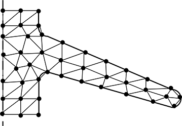
FIGURE 15.22
Modelling of HV insulator using triangular element.

15.8 FEM Examples

15.8.1 Circuit Breaker Contacts

Figure 15.23 shows the typical contact arrangement of a high-voltage circuit breaker. In order to study the arcing in the contact arrangement, it is necessary to know the electric field distribution for such arrangement. It is an axi-symmetric system. Figure 15.23a shows a triangular mesh comprising relatively larger triangular elements that could be used for FEM analysis. If the mesh size does not provide acceptable accuracy, then the discretization could be refined, as shown in Figure 15.23b. Typically, the triangles are smaller in the region where the field is expected to be high and the variation of field is non-uniform. On the other hand, in those regions where the field intensity magnitude as well as non-uniformity is lower, triangular elements of larger size are used. As a thumb rule, the element size is smaller near the boundaries and the element size becomes progressively larger as the distance from the boundary increases.

Images

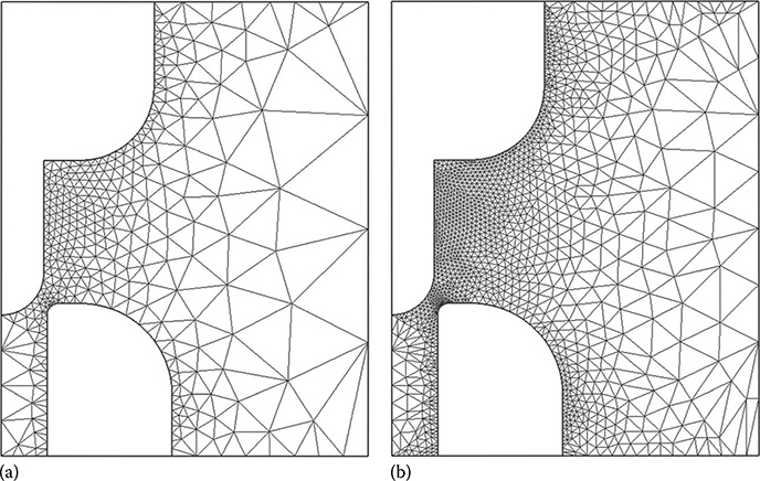
FIGURE 15.23
Modelling of circuit breaker contact using (a) coarse triangular mesh and (b) fine triangular mesh.

15.8.2 Cylindrical Insulator

A vertical cylindrical insulator with end electrodes is shown in Figure 15.24. These end electrodes also act as corona shields for high-voltage applications. This system is an axi-symmetric unbounded field region problem. In such cases, a fictitious boundary has to be considered for FEM analysis. In this example, a spherical boundary is assumed as shown. The basic rule of assuming the fictitious boundary is that the boundary should be considered at a location where the field variation is very small in space.

15.8.3 Porcelain Bushing of Transformer

Bushings are used in those cases where a live conductor has to pass through an earthed body or through a body of a different potential. In the case of transformers, the windings are normally within the tank which is earthed. Hence, the live conductor has to pass through the earthed tank for making connection to the winding. Hence, bushings are necessary for transformers. Figure 15.25 shows a typical porcelain bushing used in transformers. It is an axi-symmetric arrangement with unbounded region outside the porcelain outer cover. The central conductor has a solid insulation layer over it. The space between this solid insulation and the outer porcelain cover is filled with transformer oil. Typically, failure of bushings occurs in two different ways: (1) by means of puncture of insulation between the live conductor and the earthed tank where the radial distance between them is minimum and (2) by means of flashover that occurs along the surface of the porcelain outer cover. But in both the cases such a failure results in a terminal short circuit of the transformer, which is a major fault in any power system and is catastrophic from the viewpoint of the transformer health. Therefore, it is very important to know the electric field distribution in and around bushings, so that unwanted field concentration does not take place that may lead to failure. Typical FEM discretization of a transformer porcelain bushing is shown in Figure 15.25, which need to be refined depending on the accuracy required.

Images

FIGURE 15.24
Modelling of vertical cylindrical insulator incorporating fictitious boundary.

Images

FIGURE 15.25
Modelling of porcelain bushing of transformer.

Objective Type Questions

1. Finite element method is based on

a. Taylor series expansion

b. Fourier transform

c. Integral equation solution

d. Differential equation solution

2. In principle, finite element method is closer to

a. Charge simulation method

b. Finite difference method

c. Monte Carlo method

d. Fourier transform

3. In 2D FEM formulation, which one of the following elements is most commonly used?

a. Straight-line element

b. Ring element

c. Triangular element

d. Tetrahedral element

4. In finite element method, which one of the following is true?

a. Only conductor boundaries are discretized

b. Only dielectric boundaries are discretized

c. Both (a) and (b)

d. Entire field region is discretized

5. In FEM, if number of elements is increased, then error

a. Decreases

b. Increases

c. Remains unchanged

d. Oscillates

6. Poisson’s equation can be solved conveniently by

a. Finite element method

b. Finite difference method

c. Charge simulation method

d. Surface charge simulation method

7. In FEM formulation, within each element which one of the following parameters is considered to vary linearly, in general?

a. Electric potential

b. Electric field intensity

c. Electric flux density

d. Both (a) and (b)

8. In FEM, electric field intensity is determined by

a. Numerical integration

b. Numerical differentiation

c. Series expansion

d. Analytical expression

9. Which one of the following is the basis of variational approach in FEM formulation?

a. Energy within the field region is maximum

b. Field intensity within the field region is maximum

c. Energy within the field region is minimum

d. Field intensity within the field region is minimum

10. In FEM, higher number of elements are needed to simulate the region where field intensity

a. Varies sharply

b. Remains constant

c. Varies slowly

d. Is zero

11. FEM formulations give rise to a coefficient matrix that by property is a

a. Sparse matrix

b. Nearly full matrix

c. Diagonal matrix

d. Unit matrix

12. Which one of the following is a linear element?

a. 3-node triangular element

b. 6-node triangular element

c. 8-node quadrilateral element

d. 20-node hexahedral element

13. Which one of the following is a quadratic element?

a. 3-node triangular element

b. 6-node triangular element

c. 4-node quadrilateral element

d. 8-node hexahedral element

14. The system of simultaneous linear algebraic equations as obtained by the application of FEM in large practical problem is

a. Symmetric

b. Sparse

c. Positive definite

d. All of the above

15. Errors that arise in a typical FEM solution are

a. Discretization error

b. Formulation error

c. Numerical error

d. All of the above

16. To obtain good results in FEM analysis, the ratio between the longest and shortest sides of the element should preferably be

a. Less than 20:1

b. Less than 15:1

c. Less than 10:1

d. Less than 5:1

17. For refinement of FEM mesh, most commonly used technique is

a. To make the size of the element smaller keeping the element order constant

b. To increase the element order keeping the size of the element same

c. To decrease the size of the element along with the increase in element order

d. To re-arrange the nodes without altering the size and order of the element

18. As the size of the element decreases

a. Discretization error increases

b. Discretization error decreases

c. Formulation error decreases

d. Both (b) and (c)

19. In FEM analysis, a curved quadrilateral can be mapped to a unit square element by the use of

a. Quadratic triangular element

b. Linear quadrilateral element

c. Quadratic quadrilateral element

d. Quadratic hexahedral element

20. In FEM analysis, a hexahedron of arbitrary side length can be mapped to a unit cube element by the use of

a. Linear tetrahedral element

b. Quadratic tetrahedral element

c. Linear hexahedral element

d. Quadratic hexahedral element

21. For a finite element, if the shape function defining the geometry is of the same order as that used for defining the field variable, then the element is known as

a. Super-parametric

b. Iso-parametric

c. Sub-parametric

d. None of the above

22. In terms of the shape function used for defining the geometry as well as field variable in a finite element, the element could be

a. Super-parametric

b. Iso-parametric

c. Sub-parametric

d. All of the above

23. For a linear hexahedral element, if three shape functions are denoted as L₁ = ξ, L₂ = η and L₃ = ζ, then the fourth shape function L₄ is given by

a. ξ − η − ζ

b. ξ + η + ζ

c. 1 − ξ − η − ζ

d. 1 + ξ + η + ζ

24. For a linear triangular element, if the three shape functions are denoted as L₁, L₂ and L₃, then

a. L₁ + L₂ + L₃ = 1

b. L₁ + L₂ + L₃ = 0

c. L₁ + L₂ + L₃ = − 1

d. L₁ = L₂ + L₃

25. For a linear triangular element, if two shape functions are denoted as L₁ = ξ and L₂ = η, then the third shape function L₃ is given by

a. ξ − η

b. ξ + η

c. 1 − ξ − η

d. 1 + ξ + η

26. In FEM analysis, the approach using the minimization of potential energy is known as

a. Galerkin’s formulation

b. Variational formulation

c. Weighted residual formulation

d. None of the above

27. In high-voltage field analysis, the solution of global system of FEM equations usually gives the nodal values of

a. Electric potential

b. Electric field intensity

c. Electric flux density

d. Electric charge

Answers:

1) d;

2) b;

3) c;

4) d;

5) a;

6) a;

7) a;

8) b;

9) c;

10) a;

11) a;

12) a;

13) b;

14) d;

15) d;

16) d;

17) a;

18) d;

19) c;

20) d;

21) b;

22) d;

23) c;

24) a;

25) c;

26) b;

27) a

Bibliography

1. N. Flatabo and H. Riege, ‘Automatic calculation of electric fields’, 1st ISH Symposium, Munich, Germany, pp. 17–22, 1972.

2. B.H. McDonald and A. Wexler, ‘Finite element solution of unbounded field problems’, IEEE Transactions on Microwave Theory and Techniques, Vol. 20, No. 12, pp. 841–847, 1972.

3. O.W. Andersen, ‘Laplacian electrostatic field calculations by finite elements with automatic grid generation’, IEEE Transactions on Power Apparatus and Systems, Vol. 92, No. 5, pp. 1485–1492, 1973.

4. A. Di Napoli, C. Mazzetti and U. Ratti, A Computerized Program for the Numerical Solution of Harmonic Fields with Boundary Condition Non-Properly Defined, Compumag, Oxford, 1976.

5. O.W. Andersen, ‘Finite element solution of complex potential electric fields’, IEEE Transactions on Power Apparatus and Systems, Vol. 96, No. 4, pp. 1156–1161, 1977.

6. A. Di Napoli and C. Mazzetti, ‘Electrostatic and electromagnetic field computation for the H.V. resistive divider design’, IEEE Transactions on Power Apparatus and Systems, Vol. 98, No. 1, pp. 197–206, 1979.

7. O.W. Andersen, ‘Two stage solution of three dimensional electrostatic fields by finite differences and finite elements’, IEEE Transactions on Power Apparatus and Systems, Vol. 100, No. 8, pp. 3714–3721, 1981.

8. M.V.K. Chari, A. Konrad, J. D’Angelo and M.A. Palmo, ‘Finite element computation of three-dimensional electrostatic and magnetostatic field problems’, IEEE Transactions on Magnetics, Vol. 19, No. 6, pp. 2321–2232, 1983.

9. J.F. Hoburg and J.L. Davis, ‘A student-oriented finite element program for electrostatic potential problems’, IEEE Transactions on Education, Vol. 26, No. 4, pp. 138–142, 1983.

10. N. Burais, L. Krahenbuhl and A. Nicolas, ‘Potential distribution simulation in high voltage measurement system’, IEEE Transactions on Magnetics, Vol. 21, No. 6, pp. 2392–2395, 1985.

11. G.A. Kallio and D.E. Stock, ‘Computation of electrical conditions inside wire-duct electrostatic precipitators using a combined finite-element, finite-difference technique’, Journal of Applied Physics, Vol. 59, No. 6, pp. 1799–1806, 1986.

12. J. Penman and M.D. Grieve, ‘Self-adaptive finite-element techniques for the computation of inhomogeneous Poissonian fields’, IEEE Transactions on Industry Applications, Vol. 24, No. 6, pp. 1042–1049, 1988.

13. H. Yamashita, K. Shinozaki and E. Nakamae, ‘A boundary-finite element method to compute directly electric field intensity with high accuracy’, IEEE Transactions on Power Delivery, Vol. 3, No. 4, pp. 1754–1760, 1988.

14. O.W. Andersen, ‘PC-based field calculations for electric power applications’, IEEE Computer Applications in Power, Vol. 2, No. 4, pp. 22–25, 1989.

15. J.R. Brauer, H. Kalfaian and H. Moreines, ‘Dynamic electric fields computed by finite elements’, IEEE Transactions on Industry Applications, Vol. 25, No. 6, pp. 1088–1092, 1989.

16. R. Lakshmipathi, Y.N. Rao and G.S. Rao, ‘Computation of electrostatic field distribution in a cable by least-squares smoothing finite element method’, Communications in Applied Numerical Methods, Vol. 5, No. 1, pp. 15–22, 1989.

17. S. Cristina, G. Dinelli and M. Feliziani, ‘Numerical computation of corona space charge and V-I characteristic in DC electrostatic precipitators’, IEEE Transactions on Industry Applications, Vol. 27, No. 1, pp. 147–153, 1991.

18. C. Xiang and C. Li, ‘A finite element algorithm of plotting electric force line in two-dimensional electrostatic field computation’, IEEE Transactions on Magnetics, Vol. 28, No. 2, pp. 1789–1792, 1992.

19. H. Yamashita, E. Nakamae, T. Okano, M.S.A.A. Hammam, C. Burns and G. Adams, ‘A color graphics display of the field intensity around the insulator on 13.2 kV distribution lines’, IEEE Transactions on Electrical Insulation, Vol. 8, No. 4, pp. 1696–1702, 1993.

20. A. Wu and M.D. Driga, ‘Mathematical formulation of 2D and 3D finite and boundary element model for transient electric fields in high performance capacitors’, IEEE Transactions on Magnetics, Vol. 29, No. 1, pp. 1088–1092, 1993.

21. M. Abdel-Salam and Z. Al-Hamouz, ‘Novel finite-element analysis of space-charge modified fields’, IEEE Proceedings Science Measurement and Technology, Vol. 141, No. 5, pp. 369–378, 1994.

22. C. Xiang, J. Liu, Y. Xie, R. He, G. Zhang and C. Yang, ‘Design of insulated structure for load-ratio voltage power transformer by finite element method’, IEEE Transactions on Magnetics, Vol. 30, No. 5, pp. 2944–2947, 1994.

23. Q. Chen, A. Konrad and S. Baronijan, ‘Asymptotic boundary conditions for axi-symmetric finite element electrostatic analysis’, IEEE Transactions on Magnetics, Vol. 30, No. 6, pp. 4335–4337, 1994.

24. S. Cristina and M. Feliziani, ‘Calculation of ionized fields in DC electrostatic precipitators in the presence of dust and electric wind’, IEEE Transactions on Industry Applications, Vol. 31, No. 6, pp. 1446–1451, 1995.

25. D. Xingqi and A. Tongyi, ‘A new FEM approach for open boundary Laplace’s problem’, IEEE Transactions on Microwave Theory and Techniques, Vol. 44, No. 1, pp. 157–160, 1996.

26. A. Konrad and M. Graovac, ‘The finite element modelling of conductors and floating potentials’, IEEE Transactions on Magnetics, Vol. 32, No. 5, pp. 4329–4331, 1996.

27. S.E. Asenjo, O.N. Morales and E.A. Valdenegro, ‘Solution of low frequency complex fields in polluted insulators by means of the finite element method’, IEEE Transactions on Dielectrics and Electrical Insulation, Vol. 4, No. 1, pp. 10–16, 1997.

28. Z.M. Al-Hamouz, M. Abdel-Salam and A.M. Al-Shehri, ‘Inception voltage of corona in bipolar ionized fields-effect on corona power loss’, IEEE Transactions on Industry Applications, Vol. 34, No. 1, pp. 57–65, 1998.

29. Z.M. Al-Hamouz, M. Abdel-Salam and A. Mufti, ‘Improved calculation of finite-element analysis of bipolar corona including ion diffusion’, IEEE Transactions on Industry Applications, Vol. 34, No. 1, pp. 301–309, 1998.

30. J.Q. Feng and D.A. Hays, ‘A finite-element analysis of the electrostatic force on a uniformly charged dielectric sphere resting on a dielectric-coated electrode in a detaching electric field’, IEEE Transactions on Industry Applications, Vol. 34, No. 1, pp. 84–91, 1998.

31. D.C. Faircloth and N.L. Allen, ‘Calculations based on measurements of charge deposited by a streamer on a PTFE surface’, IEEE Transactions on Dielectrics and Electrical Insulation, Vol. 10, No. 2, pp. 291–294, 2003.

32. O.C. Zienkiewicz and R.L. Taylor, Finite Element Method, Elsevier Butterworth Heinemann, 2005.

33. S.J. Han, J. Zou, S.Q. Gu, J.L. He and J.S. Yuan, ‘Calculation of the potential distribution of high voltage metal oxide arrester by using an improved semi-analytic finite element method’, IEEE Transactions on Magnetics, Vol. 41, No. 5, pp. 1392–1395, 2005.

34. B.S. Ram, ‘Three-dimensional electrostatic field analysis of perpendicular cylinders separated by a gap’, IEEE Transactions on Power Delivery, Vol. 11, No. 1, pp. 521–522, 2006.

35. M. Boutaayamou, R.V. Sabariego and P. Dular, ‘A perturbation method for the 3D finite element modelling of electrostatically driven MEMS’, Sensors, Vol. 8, No. 2, pp. 994–1003, 2008.

36. L.N. Rossi, V.C. Silva, L.B. Martinho and J.R. Cardoso, ‘A geometrical approach of 3-D FEA for educational purposes applied to electrostatic fields’, IEEE Transactions on Magnetics, Vol. 44, No. 6, pp. 1674–1677, 2008.

37. H. Daochun, R. Jiangjun, C. Wei, L. Tianwei, W. Yuanhang and L. Jia, ‘Flashover prevention on high-altitude HVAC transmission line insulator strings’, IEEE Transactions on Dielectrics and Electrical Insulation, Vol. 16, No. 1, pp. 88–98, 2009.

38. M. Gaber, J. Pihler, M. Stegne and M. Trlep, ‘Flashover condition for a special three-electrode spark gap design’, IEEE Transactions on Power Delivery, Vol. 25, No. 1, pp. 500–507, 2010.

39. P. Maity, N. Gupta, V. Parameswaran and S. Basu, ‘On the size and dielectric properties of the interphase in epoxy-alumina nanocomposite’, IEEE Transactions on Dielectrics and Electrical Insulation, Vol. 17, No. 6, pp. 1665–1675, 2010.

40. N. Farnoosh, K. Adamiak and G.S.P. Castle, ‘3-D numerical simulation of particle concentration effect on a single-wire ESP performance for collecting poly-dispersed particles’, IEEE Transactions on Dielectrics and Electrical Insulation, Vol. 18, No. 1, pp. 211–220, 2011.

41. X.B. Bian, D.Y. Yu, M. Xiaobo, M. Macalpine, W. Liming, G. Zhicheng, Y. Wenjun and Z. Shuzhen, ‘Corona-generated space charge effects on electric field distribution for an indoor corona cage and a monopolar test line’, IEEE Transactions on Dielectrics and Electrical Insulation, Vol. 18, No. 5, pp. 1767–1778, 2011.

42. W.N. Fu, S.L. Ho, S. Niu and J.G. Zhu, ‘Comparison study of finite element methods to deal with floating conductors in electric field’, IEEE Transactions on Magnetics, Vol. 48, No. 2, pp. 351–354, 2012.

..................Content has been hidden....................

You can't read the all page of ebook, please click here login for view all page.

Table of Contents for 15. Numerical Computation of High-Voltage Field by Finite Element Method

Create new playlist

Sign In

Sign Up

PROBLEM 15.1

PROBLEM 15.2

PROBLEM 15.3

PROBLEM 15.4

Answers:

Table of Contents for
15. Numerical Computation of High-Voltage Field by Finite Element Method