3. Orthogonal Coordinate Systems

Search in book...
Toggle Font Controls
Create new playlist

Name your new playlist

Playlist description (optional)
Sign In

Email address

Password

Forgot Password?

or

Continue with Facebook

Continue with Google
Sign Up

Full Name

Email address

Confirm Email Address

Password

or

Continue with Facebook

Continue with Google

ABSTRACT The purpose of this chapter is to present coordinate systems in such a way that it improves the ability of readers to use them to describe the electric field in a better way. The goal is to put forward the coordinate system as a useful language for describing, visualizing and understanding the concepts that are central to electric field analysis. Many mathematical operators related to electric field analysis have simple forms in Cartesian coordinates and are easy to remember and evaluate. In fact, all the problems could be solved using the Cartesian coordinate system. However, the resulting expressions might be unnecessarily complex. While dealing with problems that have high degree of symmetry, it is helpful to use a coordinate system that exploits the symmetry. As a result, it is useful to have a general method for expressing mathematical operators in non-Cartesian forms. Orthogonal curvilinear coordinate system is a useful approach by which the matching of the symmetry of a given physical configuration could be done and simplified mathematical models could be built to clarify the field concepts clearly.

3.1 Basic Concepts

The concept that unifies the different coordinate systems is surfaces of constant coordinates. It means that an equation of the form (coordinate = value) defines a surface. In order to specify a point uniquely in a three-dimensional space, three different types of surfaces are needed. The values associated with the three constant coordinate surfaces that intersect at a specific point are the three coordinates, which uniquely define that point.

Consider that three surfaces are defined by three functions f₁, f₂ and f₃, respectively, in a three-dimensional space. The coordinate, that is, the value, that describes a surface could be defined by the equation f_i = u_i. Here, u is introduced to represent a generalized coordinate. In the stated equation, u_i refers to one of the coordinates in a particular system. Thus, the three values (u₁,u₂,u₃) define a point, where the three surfaces defined by Equation 3.1 intersect. These three values (u₁,u₂,u₃) are then called the coordinates of that particular point.

$f_{1} = u_{1}, f_{2} = u_{2} and f_{3} = u_{3} (3.1)$

The three functions, however, could not be chosen arbitrarily. The three functions are to be chosen in such a way that for any choice of the three coordinates (u₁,u₂,u₃), the three surfaces generated by Equation 3.1 will intersect only at one point. It will ensure that a given set of three coordinate values (u₁,u₂,u₃) always specifies only one point in space. Moreover, the constant coordinate surfaces are always perpendicular to each other, that is, orthogonal, at the point where they intersect. The intersection of any two constant coordinate surfaces defines a coordinate curve.

3.1.1 Unit Vector

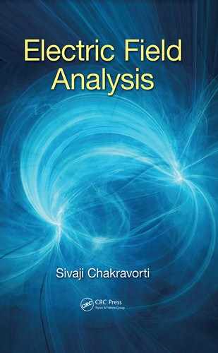
An important concept associated with coordinate system is unit vector. It will be easy to understand the concept if it is explained with the help of a specific example involving the Cartesian coordinate system, as shown in Figure 3.1. Each value of z, for example, z₁, z₂ or z₃, defines a plane normal to the z-axis. The unit vector $\hat{k}$ is defined in such a way that it is normal to all such z = constant planes and points in the direction of the planes with increasing values of z, as shown in Figure 3.1. The magnitude of the vector $\hat{k}$ is taken as unity. The other two unit vectors in the Cartesian coordinate system could be visualized in the same manner.

In a generalized manner, the properties of the unit vector associated with a constant coordinate surface defined by the function f_i are as follows: (1) it is perpendicular to the surface f_i = u_i at any point (u₁,u₂,u₃); (2) it points in the direction of the surfaces with increasing value of u_i and (3) it is one unit in magnitude. Orthogonality of the constant coordinate surfaces, as discussed earlier, demands that the dot product of any two different unit vectors will always be zero. Conversely, the dot product of two same unit vectors, for example, $\hat{k} \cdot \hat{k}$ , will always be 1.

Images

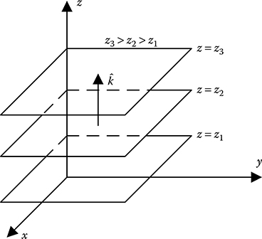
FIGURE 3.1
The unit vector $\hat{k}$ .

3.1.2 Right-Handed Convention

Because three constant coordinate surfaces are involved in determining the coordinates of any point, the question that arises is in which order the three coordinates are to be mentioned while specifying a point. In this context, the choice of the first coordinate (u₁) or surface (f₁) is arbitrary. Once f₁ is chosen, then the order in which the other two constant coordinate surfaces f₂ and f₃ is to be taken is determined by the right-handed system as governed by the definition of vector cross product. In other words, the cross product of the first and second unit vectors must be equal to the third unit vector.

This right-handed property of the coordinate system is an arbitrary convention. But once that choice is made for one coordinate system, it has to be followed for all other coordinate systems to ensure that the expressions for the laws of electric field have the same form in all the coordinate systems.

3.1.3 Differential Distance and Metric Coefficient

The constant coordinate surfaces could be of many different types. The simplest of them is constant distance surfaces for which the differential change du_i in the coordinate u_i is the same as the differential distance dl_i between the surfaces f_i = u_i and f_i = u_i + d u_i. However, there are other types of surfaces such as constant angle surfaces, in which case the differential distance is related to differential coordinate (angle) change as

$d l_{i} = h_{i} d u_{i} = h_{i} d θ_{i} (3.2)$

where:

The scale factor h_i is the corresponding radius

The scale factors for each of the coordinate system are called the metric coefficients of the respective coordinate system. The three metric functions of any coordinate system (h₁,h₂,h₃) constitute a unique set and hence are often known as the signature of a coordinate system. Metric coefficients are also very important in writing the vector operators in the general orthogonal curvilinear coordinate system, as will be explained in Section 3.5.

3.1.4 Choice of Origin

A basic element of any coordinate system is the choice of origin. If any object or any arrangement is given, then any point within the object or within the whole arrangement could be chosen as origin.

From the earlier discussions, it is clear that the same point will have very different coordinates when defined in different coordinate systems. Therefore, the question that needs to be answered is that whether there is any property of the position of the point that remains the same in different coordinate systems. The answer to this question is that the distance of the point from the origin remains the same in all the coordinate systems if the origin is kept the same in all the cases. As a logical extension, it may be stated that the distance between any two points remains the same no matter how their coordinates are defined in any coordinate system.

3.2 Cartesian Coordinate System

The invention of Cartesian coordinates in the seventeenth century by the French mathematician René Descartes revolutionized mathematics by providing the first systematic link between Euclidean geometry and algebra. In this coordinate system, the three constant coordinate surfaces are defined by Equation 3.3

$f_{1} = x, f_{2} = y, f_{3} = z (3.3)$

Figure 3.2 shows such constant coordinate surfaces, which are three planes. Cartesian coordinate system has the unique feature that all the three constant coordinate surfaces are constant distance surfaces.

Each point P in space is then assigned a triplet of values (x,y,z), the so-called Cartesian coordinates of that point. The ranges of the values of three coordinates are −∞ < x < ∞, −∞ < y < ∞ and −∞ < z < ∞. Coordinates can be

Images

FIGURE 3.2
Constant coordinate surfaces in the Cartesian coordinate system.

defined as the positions of the normal projections of the point onto three mutually perpendicular constant coordinate surfaces passing through the origin, expressed as signed distances from the origin.

In the Cartesian coordinate system, three mutually perpendicular axes are commonly defined as follows. The intersection of two mutually perpendicular planes y = constant and z = constant passing through the origin gives a coordinate curve, which is a straight line. This line is then defined as the x-axis. Similarly, the intersections of other two pairs of mutually perpendicular constant coordinate planes passing through origin define the y- and z-axes.

The unit vector $\hat{i}$ is perpendicular to all the surfaces described by x = constant and points in the direction of increasing value of x-coordinate. In the same manner, unit vectors $\hat{j}$ and $\hat{k}$ are defined in y- and z-directions, respectively. Another unique feature of the Cartesian coordinate system is that the directions of the three unit vectors remain the same irrespective of the location of the point in space. The orthogonality of the Cartesian coordinate system is defined by Equation 3.4

$\hat{i} \cdot \hat{j} = 0, \hat{j} \cdot \hat{k} = 0, \hat{k} \cdot \hat{i} = 0 (3.4)$

and the right handedness is defined by Equation 3.5

$\hat{i} \times \hat{j} = \hat{k}, \hat{j} \times \hat{k} = \hat{i}, \hat{k} \times \hat{i} = \hat{j} (3.5)$

As shown in Figure 3.3, the differential line element in the Cartesian coordinate system is given by Equation 3.6

$d \vec{l} = d l_{1} \hat{i} + d l_{2} \hat{j} + d l_{3} \hat{k} = d x \hat{i} + d y \hat{j} + d z \overset{\leftarrow}{k} (3.6)$

As shown in Figure 3.4, the differential area element corresponding to the surface of a differential cubical volume is given by Equation 3.7

Images

FIGURE 3.3
Differential line element in the Cartesian coordinate system.

Images

FIGURE 3.4
Differential area and volume elements in the Cartesian coordinate system.

$d {\vec{A}}_{x y} = d l_{1} d l_{2} \hat{k} = d x d y \hat{k} (3.7)$

As shown in Figure 3.4, the differential volume element is given by Equation 3.8

$d V = d l_{1} d l_{2} d l_{3} = d x d y d z (3.8)$

As depicted in Equation 3.6 the differential distance in x-direction is dl₁ = dx = h₁dx, that is, h₁ = 1. Similarly, in y- and z-directions, h₂ = h₃ = 1. The metric coefficients of the Cartesian coordinate system are, therefore, h₁ = 1, h₂ = 1 and h₃ = 1.

3.3 Cylindrical Coordinate System

Cylindrical coordinates are an alternate way of describing points in a three-dimensional space. In this coordinate system, one of the rectangular coordinate planes, namely, the x–y plane, as described by the Cartesian coordinate system, is replaced by a polar plane. In the cylindrical coordinate system, everything is measured with respect to a fixed point called the pole and an axis called the polar axis. The pole is the equivalent to the origin in the Cartesian coordinate system and the polar axis corresponds to the positive direction of the x-axis. The cylindrical coordinates of a point are then the ordered triplet (r,θ,z), as defined in Figure 3.5.

As shown in Figure 3.5, r is the distance from the pole to the projection of the point P on the polar plane, that is, the x–y plane passing through the pole, θ is the azimuthal angle, that is, the angle from the polar axis spinning around the z-axis in counter-clockwise direction, and z is the vertical height from the polar plane. The ranges of the values of the three coordinates are 0 ≤ r < ∞, 0 ≤ θ ≤ 2π and −∞ < z < ∞.

Images

FIGURE 3.5
Depiction of cylindrical coordinates of a point.

In the cylindrical coordinate system, the three constant coordinate surfaces are defined by Equation 3.9

$f_{1} = r, f_{2} = θ, f_{3} = z (3.9)$

Figure 3.6 shows the three constant coordinate surfaces in the cylindrical coordinate system. Out of these three surfaces, the first and the third surfaces, namely, f₁ = r and f₃ = z, are constant distance surfaces, whereas the second one, that is, f₂ = θ, is a constant angle surface. As shown in Figure 3.6, the surfaces θ = constant and z = constant are planes, whereas the surface r = constant is a cylindrical surface.

In this coordinate system, two unit vectors are defined on the x–y plane. The unit vector û_r points in the direction of increasing r, that is, radially outwards from the z-axis and the unit vector û_θ points in the direction of increasing θ, that is, it points in the direction of the tangent to the circle of radius r in the counter-clockwise sense. The third unit vector û_z points in the direction of increasing z, that is, vertically upwards from the x–y plane. The unit vectors are shown in Figure 3.5. The orthogonality of cylindrical coordinate system is defined by Equation 3.10

${\hat{u}}_{r} \cdot {\hat{u}}_{θ} = 0, {\hat{u}}_{θ} \cdot {\hat{u}}_{z} = 0, {\hat{u}}_{z} \cdot {\hat{u}}_{r} = 0 (3.10)$

and the right handedness is defined by Equation 3.11

${\hat{u}}_{r} \times {\hat{u}}_{θ} = {\hat{u}}_{z}, {\hat{u}}_{θ} \times {\hat{u}}_{z} = {\hat{u}}_{r}, {\hat{u}}_{z} \times {\hat{u}}_{r} = {\hat{u}}_{θ} (3.11)$

Images

FIGURE 3.6
Constant coordinate surfaces in the cylindrical coordinate system.

Images

FIGURE 3.7
Unit vectors at different points in the cylindrical coordinate system.

Unlike the Cartesian system, in the cylindrical coordinate system, the directions of all the three unit vectors do not remain the same as one moves around the space. As shown in Figure 3.7, the directions of the unit vectors û_r and û_θ get changed at different points in space keeping û_z unchanged.

As shown in Figure 3.8, the differential line element in the cylindrical coordinate system is given by Equation 3.12

$d \vec{l} = d l_{1} {\hat{u}}_{r} + d l_{2} {\hat{u}}_{θ} + d l_{3} {\hat{u}}_{z} = d r {\hat{u}}_{r} + r d_{θ} {\hat{u}}_{θ} + d z {\hat{u}}_{z} (3.12)$

Images

FIGURE 3.8
Differential line element in the cylindrical coordinate system.

Images

FIGURE 3.9
Differential area element on the cylinder surface in the cylindrical coordinate system.

As shown in Figure 3.9, in the cylindrical coordinate system, the differential area element on the surface of a cylinder of radius r is given by Equation 3.13

$d {\vec{A}}_{θ z} = d l_{2} d l_{3} {\hat{u}}_{r} = r d θ d z {\hat{u}}_{r} (3.13)$

and the differential area element on the surface of a disc in the x–y plane, as shown in Figure 3.10, is given by Equation 3.14

$d {\vec{A}}_{r θ} = d l_{1} d l_{2} {\hat{u}}_{z} = d r r d θ {\hat{u}}_{z} (3.14)$

Images

FIGURE 3.10
Differential area element on the disc surface in the cylindrical coordinate system.

Images

FIGURE 3.11
Differential volume element of a cylinder in the cylindrical coordinate system.

As shown in Figure 3.11, the differential volume element is given by Equation 3.15

$d V = d l_{1} d l_{2} d l_{3} = d r r d θ d z (3.15)$

As depicted in Equation 3.12, the differential distance in r-direction is dl₁ = dr = h₁dr, that is, h₁ = 1, in θ-direction, it is dl₂ = rdθ = h₂dθ, that is, h₂ = r and in z-direction, it is dl₃ = dz = h₃dz, that is, h₃ = 1. The metric coefficients of cylindrical coordinate system are, therefore, h₁ = 1, h₂ = r and h₃ = 1.

3.4 Spherical Coordinate System

Spherical coordinates are particularly useful for analyzing fields having spherical symmetry. In the spherical coordinate system, the coordinates of any point in space are the ordered triplet (r,θ,ϕ), as shown in Figure 3.12. The coordinate r measures the radial distance from the origin to the point P. The coordinate θ is the angle that the r vector makes with the positive direction of the z-axis, whereas the coordinate ϕ is the azimuthal angle with respect to the positive direction of the x-axis spinning around the z-axis in counterclockwise sense. The angle ϕ is defined on the x–y plane. The ranges of the values of the three coordinates are 0 ≤ r < ∞, 0 ≤ θ ≤ π and 0 ≤ ϕ ≤ 2π.

In the spherical coordinate system, the three constant coordinate surfaces are defined by Equation 3.16

$f_{1} = r, f_{2} = θ, f_{3} = ϕ (3.16)$

Figure 3.13 shows the three constant coordinate surfaces in the spherical coordinate system. Out of these three surfaces, the first surface, namely, f₁ = r, is a constant distance surface, whereas the other two surfaces, that is, f₂ = θ and f₃ = ϕ, are constant angle surfaces. As shown in Figure 3.13, r = constant is a spherical surface, θ = constant is a conical surface and ϕ = constant is a plane.

In this coordinate system, the unit vector û_r points in the direction of increasing r, that is, radially outwards from the origin. The unit vector û_θ points in the direction of increasing θ along the tangent to a circle of radius r in the plane containing the z-axis and the r vector. The unit vector û_ϕ points

Images

FIGURE 3.12
Depiction of spherical coordinates of a point.

Images

FIGURE 3.13
Constant coordinate surfaces in the spherical coordinate system.

in the direction of increasing ϕ along the tangent to a circle in the x–y plane, which is centred on the z-axis. The unit vectors are shown in Figure 3.12. The orthogonality of the spherical coordinate system is defined by Equation 3.17

${\hat{u}}_{r} \cdot {\hat{u}}_{θ} = 0, {\hat{u}}_{θ} \cdot {\hat{u}}_{ϕ} = 0, {\hat{u}}_{ϕ} \cdot {\hat{u}}_{r} = 0 (3.17)$

and the right handedness is defined by Equation 3.18

${\hat{u}}_{r} \times {\hat{u}}_{θ} = {\hat{u}}_{ϕ}, {\hat{u}}_{θ} \times {\hat{u}}_{ϕ} = {\hat{u}}_{r}, {\hat{u}}_{ϕ} \times {\hat{u}}_{r} = {\hat{u}}_{θ} (3.18)$

Similar to the cylindrical coordinate system, in the spherical coordinate system, the directions of all the three unit vectors do not remain the same as one move around the space. As shown in Figure 3.14, the directions of all the three unit vectors û_r, û_θ and û_ϕ get changed at different points in space. As shown in Figure 3.15, the differential line element in the spherical coordinate system is given by Equation 3.19

$d \vec{l} = d l_{1} {\hat{u}}_{r} + d l_{2} {\hat{u}}_{θ} + d l_{3} {\hat{u}}_{ϕ} = d r {\hat{u}}_{r} + r d θ {\hat{u}}_{θ} + r \sin θ d ϕ {\hat{u}}_{ϕ} (3.19)$

As shown in Figure 3.16, in the spherical coordinate system, the differential area element on the surface of a sphere of radius r is given by Equation 3.20

$d {\vec{A}}_{θ ϕ} = d l_{2} d l_{3} {\hat{u}}_{r} = (r d θ) (r \sin θ d ϕ) {\hat{u}}_{r} = r^{2} \sin θ d θ d ϕ {\hat{u}}_{r} (3.20)$

Images

FIGURE 3.14
Unit vectors at different points in the spherical coordinate system.

Images

FIGURE 3.15
Differential line element in the spherical coordinate system.

Images

FIGURE 3.16
Differential area element on the sphere surface in the spherical coordinate system.

As shown in Figure 3.17, the differential volume element is given by Equation 3.21

$d V = d l_{1} d l_{2} d l_{3} = (d r) (r d θ) (r \sin θ d ϕ) = r^{2} \sin θ d r d θ d ϕ (3.21)$

As depicted in Equation 3.19, the differential distance in r-direction is dl₁ = dr = h₁dr, that is, h₁ = 1, in θ-direction, it is dl₂ = rdθ = h₂dθ, that is, h₂ = r and in ϕ-direction, it is dl₃ = r sin θdϕ = h₃dϕ, that is, h₃ = r sin θ. Therefore, the metric coefficients of spherical coordinate system are h₁ = 1, h₂ = r and h₃ = r sin θ.

3.5 Generalized Orthogonal Curvilinear Coordinate System

From the discussions of the previous sections, it may be seen that a major hindrance in treating the three commonly used orthogonal coordinate systems, namely, Cartesian, cylindrical and spherical coordinate systems, on an equal footing is that the unit vectors are not the best way to visualize these three coordinate systems. In this context, a generalized orthogonal curvilinear coordinate system provides insight for useful linkage between such orthogonal coordinate systems. Generalized orthogonal curvilinear coordinate system emphasizes on the similarities between different orthogonal coordinate systems rather than highlighting their differences. Thus, the definition and utilization of generalized orthogonal curvilinear coordinate system is very important for the proper understanding of the formulation and solution of electric field problems.

Images

FIGURE 3.17
Differential volume element of a sphere in the spherical coordinate system.

Consider that f(x,y,z) = u is a function of three independent space variables x,y,z in the Cartesian coordinate system that specify a surface characterized by the constant parameter u. Setting such function equal to three different constant parameters u₁, u₂ and u₃ defines three different surfaces as follows:

$f_{1} (x, y, z) = u_{1}, f_{2} (x, y, z) = u_{2} and f_{3} (x, y, z) = u_{3} (3.22)$

Considering that these three surfaces are orthogonal, they intersect in space only at one point. In other words, any point in space could be uniquely defined by a set of values of the three parameters (u₁,u₂,u₃), which are then called the orthogonal curvilinear coordinates of the point being defined. The constant coordinate surfaces for a generalized orthogonal curvilinear coordinate system are shown in Figure 3.18.

As shown in Figure 3.18, the unit vectors â₁, â₂ and â₃ are normal to the surfaces u₁ = constant, u₂ = constant and u₃ = constant, respectively, and point towards the increasing values of the coordinates u₁, u₂ and u₃, respectively. The orthogonality of the generalized curvilinear coordinate system is defined by Equation 3.23

${\hat{a}}_{1} \cdot {\hat{a}}_{2} = 0, {\hat{a}}_{2} \cdot {\hat{a}}_{3} = 0, {\hat{a}}_{3} \cdot {\hat{a}}_{1} = 0 (3.23)$

Images

FIGURE 3.18
Constant coordinate surfaces in the generalized orthogonal curvilinear coordinate system.

and the right handedness is defined by Equation 3.24

${\hat{a}}_{1} \times {\hat{a}}_{2} = {\hat{a}}_{3}, {\hat{a}}_{2} \times {\hat{a}}_{3} = {\hat{a}}_{1}, {\hat{a}}_{3} \times {\hat{a}}_{1} = {\hat{a}}_{2} (3.24)$

As shown in Figure 3.19, the surfaces u = u₁ and u = u₁ + du₁ are separated by a differential length element dl₁, which is normal to the surface u = u₁, where dl₁ = h₁(u₁,u₂,u₃)du₁. The scale factor or the metric coefficient h₁ is a function of the three curvilinear coordinates (u₁,u₂,u₃). The other two metric coefficients, that is, h₂(u₁,u₂,u₃) and h₃(u₁,u₂,u₃), are also similarly defined.

As shown in Figure 3.19, the differential line element in the generalized orthogonal curvilinear coordinate system is given by Equation 3.25

$d \vec{l} = d l_{1} {\hat{a}}_{1} + d l_{2} {\hat{a}}_{2} + d l_{3} {\hat{a}}_{3} = h_{1} d u_{1} {\hat{a}}_{1} + h_{2} d u_{2} {\hat{a}}_{2} + h_{3} d u_{3} {\hat{a}}_{3} (3.25)$

As shown in Figure 3.19, the differential area elements in the generalized orthogonal curvilinear coordinate system are given by Equation 3.26

$\begin{matrix} d {\vec{A}}_{12} = (h_{1} d u_{1}) (h_{2} d u_{2}) {\hat{a}}_{3} = h_{1} h_{2} d u_{1} d u_{2} {\hat{a}}_{3} \\ d {\vec{A}}_{23} = (h_{2} d u_{2}) (h_{3} d u_{3}) {\hat{a}}_{1} = h_{2} h_{3} d u_{2} d u_{3} {\hat{a}}_{1} \\ d {\vec{A}}_{31} = (h_{3} d u_{3}) (h_{1} d u_{1}) {\hat{a}}_{2} = h_{3} h_{1} d u_{3} d u_{1} {\hat{a}}_{2} \end{matrix} (3.26)$

and the differential volume element in generalized orthogonal curvilinear coordinate system is given by Equation 3.27

Images

FIGURE 3.19
Differential line, area and volume elements in the generalized orthogonal curvilinear coordinate system.

$d V = (h_{1} d u_{1}) (h_{2} d u_{2}) (h_{3} d u_{3}) = h_{1} h_{2} h_{3} d u_{1} d u_{2} d u_{3} (3.27)$

In the light of the generalized orthogonal curvilinear coordinate system, the three commonly used orthogonal coordinate systems could be summarized as in Table 3.1.

Recall that the metric coefficients were earlier stated to be functions of the coordinates (u₁,u₂,u₃). Table 3.1 clearly shows such dependence of the metric coefficients on the respective coordinates in cylindrical and spherical coordinate systems. Cartesian coordinate system is unique in the sense that its metric coefficients are constant.

TABLE 3.1
Characterization of Orthogonal Coordinate Systems

Orthogonal Coordinate System	Coordinates	Unit Vectors	Metric Coefficients
Generalized	(u₁,u₂,u₃)	$({\hat{a}}_{1}, {\hat{a}}_{2}, {\hat{a}}_{3})$	(h₁,h₂,h₃)
Cartesian	(x,y,z)	$(\hat{i}, \hat{j}, \hat{k})$	(1,1,1)
Cylindrical	(r,θ,z)	$({\hat{u}}_{r}, {\hat{u}}_{θ}, {\hat{u}}_{z})$	(1,r,1)
Spherical	(r,θ,ϕ)	$({\hat{u}}_{r}, {\hat{u}}_{θ}, {\hat{u}}_{ϕ})$	(1, r,r, sin θ)

3.6 Vector Operations

In field analysis, it is often required to perform vector operations to get vector and scalar derivatives of scalar and vector fields, which are scalar and vector functions of position, respectively. Most commonly used vector operations are gradient, divergence, curl and Laplacian. It is possible to get expressions for all these vector operations in the generalized orthogonal curvilinear coordinate system. In order to get such expressions, consider an arbitrary scalar field like electric potential or temperature as U(u₁, u₂, u₃) and an arbitrary vector field like electric flux density or force as

$\vec{S} = S_{1} (u_{1}, u_{2}, u_{3}) {\hat{a}}_{1} + S_{2} (u_{1}, u_{2}, u_{3}) {\hat{a}}_{2} + S_{3} (u_{1}, u_{2}, u_{3}) {\hat{a}}_{3} (3.28)$

3.6.1 Gradient

In electric field analysis, a common application of gradient operation is to determine electric field intensity from the knowledge of electric potential. In order to understand this concept clearly, a change dU in the scalar function U is expressed in terms of the changes in differential distances dl₁, dl₂ and dl₃ in the generalized orthogonal curvilinear coordinate system as follows:

$d U = \frac{\partial U}{\partial l_{1}} d l_{1} + \frac{\partial U}{\partial l_{2}} d l_{2} + \frac{\partial U}{\partial l_{3}} d l_{3} (3.29)$

Introducing the differential distance as $d \vec{l} = d l_{1} {\hat{a}}_{1} + d l_{2} {\hat{a}}_{2} + d l_{3} {\hat{a}}_{3}$ , the above equation could be rewritten as follows:

$d U = (\frac{\partial U}{\partial l_{1}} {\hat{a}}_{1} + \frac{\partial U}{\partial l_{2}} {\hat{a}}_{2} + \frac{\partial U}{\partial l_{3}} {\hat{a}}_{3}) \cdot (d l_{1} {\hat{a}}_{1} + d l_{2} {\hat{a}}_{2} + d l_{3} {\hat{a}}_{3}) = \vec{\nabla} U \cdot d \vec{l} (3.30)$

where:

$\vec{\nabla} U = \frac{\partial U}{\partial l_{1}} {\hat{a}}_{1} + \frac{\partial U}{\partial l_{2}} {\hat{a}}_{2} + \frac{\partial U}{\partial l_{3}} {\hat{a}}_{3} = \frac{1}{h_{1}} \frac{\partial U}{\partial u_{1}} {\hat{a}}_{1} + \frac{1}{h_{2}} \frac{\partial U}{\partial u_{2}} {\hat{a}}_{2} + \frac{1}{h_{3}} \frac{\partial U}{\partial u_{3}} {\hat{a}}_{3} (3.31)$

Equation 3.30 indicates that the change dU in the scalar function U over the differential distance dl at any point in space is maximum when $\vec{\nabla} U$ and $d \vec{l}$ are in the same direction. In other words, the magnitude of the vector $\vec{\nabla} U$ , which is the spatial derivative of the scalar function U and is called the gradient of U, is equal to the maximum value of dU/dl and it is in the direction in which dU/dl is maximum.

With the help of the metric coefficients and other parameters mentioned in Table 3.1, the gradient function can be written in different orthogonal coordinate systems as detailed below:

Cartesian coordinate system:

$\vec{\nabla} U = \frac{\partial U}{\partial x} \hat{i} + \frac{\partial U}{\partial y} \hat{j} + \frac{\partial U}{\partial z} \hat{k} (3.32)$

Cylindrical coordinate system:

$\vec{\nabla} U = \frac{\partial U}{\partial r} {\hat{u}}_{r} + \frac{1}{r} \frac{\partial U}{\partial θ} {\hat{u}}_{θ} + \frac{\partial U}{\partial z} {\hat{u}}_{z} (3.33)$

Spherical coordinate system:

$\vec{\nabla} U = \frac{\partial U}{\partial r} {\hat{u}}_{r} + \frac{1}{r} \frac{\partial U}{\partial θ} {\hat{u}}_{θ} + \frac{l}{r \sin θ} \frac{\partial U}{\partial ϕ} {\hat{u}}_{ϕ} (3.34)$

3.6.2 Del Operator

Equation 3.30 introduces a vector differential operator $\vec{\nabla}$ such that when $\vec{\nabla}$ is applied on a scalar function, it results into a vector function. Such vector operation is called gradient.

From Equation 3.31

$\begin{matrix} \vec{\nabla} U & = \frac{1}{h_{1}} \frac{\partial U}{\partial u_{1}} {\hat{a}}_{1} + \frac{1}{h_{2}} \frac{\partial U}{\partial u_{2}} {\hat{a}}_{2} + \frac{1}{h_{3}} \frac{\partial U}{\partial u_{3}} {\hat{a}}_{3} \\ = (\frac{1}{h_{1}} \frac{\partial}{\partial u_{1}} {\hat{a}}_{1} + \frac{1}{h_{2}} \frac{\partial}{\partial u_{2}} {\hat{a}}_{2} + \frac{1}{h_{3}} \frac{\partial}{\partial u_{3}} {\hat{a}}_{3}) U \\ so that \vec{\nabla} & = (\frac{1}{h_{1}} \frac{\partial}{\partial u_{1}} {\hat{a}}_{1} + \frac{1}{h_{2}} \frac{\partial}{\partial u_{2}} {\hat{a}}_{2} + \frac{1}{h_{3}} \frac{\partial}{\partial u_{3}} {\hat{a}}_{3}) \end{matrix} (3.35)$

It has been discussed in Chapter 2 that when $\vec{\nabla}$ is applied on a vector function as scalar or dot product, then it results into a scalar function and such operation is called divergence. On the other hand, when $\vec{\nabla}$ is operated on a vector function with vector or cross product, then it results into another vector function and this operation is called curl.

3.6.3 Divergence

In electric field analysis, divergence is used to relate electric field with the source, that is, the charges, as given by the differential form of Gauss’s law.

It has already been discussed in Chapter 2 that the divergence of a vector field $\vec{S}$ could be evaluated by finding the net flux coming out per unit volume. In this context, consider the differential volume element dV = (dl₁dl₂dl₃), as shown in Figure 3.20. Consider that the point O is located at the centre of the volume element dV and also that the vector $\vec{S}$ is known at the point O.

Images

FIGURE 3.20
Divergence in the generalized orthogonal curvilinear coordinate system.

The points 1 and 2 are the midpoints of the surfaces ABCD and EFGH, respectively, which are normal to u₁ direction. Therefore, along the line 1-O-2 the derivatives of S₁, which is the u₁ component of $\vec{S}$ , with respect to u₁, will be finite, whereas the derivative of S₁ with respect to u₂ and u₃ will be zero, as S₁ is orthogonal to u₂ and u₃. Considering the differential distance dl₁ between the two surfaces under reference, namely, ABCD and EFGH, S₁ at the points 1 and 2 can be evaluated from the knowledge of S₁ at O with the help of Taylor series. Noting that the distances between O and both the points 1 and 2 are dl₁/2, from the Taylor series expansion, it can be written neglecting higher order terms as follows:

$S_{1} |_{1} = S_{1} - \frac{\partial S_{1}}{\partial l_{1}} \frac{d l_{1}}{2}$ (as the distance from O to 1 is in the negative sense of u₁)
$S_{1} |_{2} = S_{1} + \frac{\partial S_{1}}{\partial l_{1}} \frac{d l_{1}}{2}$ (as the distance from O to 2 is in the positive sense of u₁)

where:

S₁ stands for the value of S₁ at O

Therefore,

$\begin{matrix} S_{1} |_{1} & = S_{1} - \frac{\partial S_{1}}{h_{1} \partial u_{1}} \frac{h_{1} d u_{1}}{2} = S_{1} - \frac{\partial S_{1}}{\partial u_{1}} \frac{d u_{1}}{2} \\ and S_{1} |_{2} & = S_{1} + \frac{\partial S_{1}}{h_{1} \partial u_{1}} \frac{h_{1} d u_{1}}{2} = S_{1} + \frac{\partial S_{1}}{\partial u_{1}} \frac{d u_{1}}{2} \end{matrix}$

The area of the surface ABCD is given by dl₂dl₃ = h₂h₃du₂du₃. Therefore, the flux of $\vec{S}$ going into the differential volume through the surface ABCD in the u₁ direction is given by

$\begin{matrix} d ψ_{A B C D} & = (S_{1} h_{2} h_{3} d u_{2} d u_{3}) - \frac{\partial (S_{1} h_{2} h_{3} d u_{2} d u_{3})}{\partial u_{1}} \frac{d u_{1}}{2} \\ = (S_{1} h_{2} h_{3} d u_{2} d u_{3}) - \frac{\partial (S_{1} h_{2} h_{3})}{\partial u_{1}} \frac{d u_{1} d u_{2} d u_{3}}{2} \end{matrix}$

as (h₁, h₂, h₃) are functions of (u₁, u₂, u₃), the product h₂h₃ is kept within the partial derivative term.

Similarly, the flux of $\vec{S}$ coming out of the surface EFGH in the u₁ direction is given by

$\begin{matrix} d ψ_{E F G H} & = (S_{1} h_{2} h_{3} d u_{2} d u_{3}) + \frac{\partial (S_{1} h_{2} h_{3} d u_{2} d u_{3})}{\partial u_{1}} \frac{d u_{1}}{2} \\ = (S_{1} h_{2} h_{3} d u_{2} d u_{3}) + \frac{\partial (S_{1} h_{2} h_{3})}{\partial u_{1}} \frac{d u_{1} d u_{2} d u_{3}}{2} \end{matrix}$

Hence, the net flux coming out of the differential volume in the u₁ direction is given by

$d ψ_{1} = d ψ_{E F G H} - d ψ_{A B C D} = \frac{\partial (S_{1} h_{2} h_{3})}{\partial u_{1}} d u_{1} d u_{2} d u_{3} (3.36)$

Therefore, considering all the three directions, that is, u₁, u₂ and u₃ directions, the net flux coming out of the volume dV is

$ψ_{d V} = [\frac{\partial (S_{1} h_{2} h_{3})}{\partial u_{1}} + \frac{\partial (S_{2} h_{3} h_{1})}{\partial u_{2}} + \frac{\partial (S_{3} h_{1} h_{2})}{\partial u_{3}}] d u_{1} d u_{2} d u_{3} (3.37)$

Therefore, the divergence of $\vec{S}$ , which is the net flux coming out per unit volume, is given by

$\begin{matrix} d i v \vec{S} = \frac{ψ_{d V}}{d V} = \frac{1}{d l_{1} d l_{2} d l_{3}} [\frac{\partial (S_{1} h_{2} h_{3})}{\partial u_{1}} + \frac{\partial (S_{2} h_{3} h_{1})}{\partial u_{2}} + \frac{\partial (S_{3} h_{1} h_{2})}{\partial u_{3}}] d u_{1} d u_{2} d u_{3} \\ or, d i v \vec{S} = \frac{1}{h_{1} h_{2} h_{3} d u_{1} d u_{2} d u_{3}} [\frac{\partial (S_{1} h_{2} h_{3})}{\partial u_{1}} + \frac{\partial (S_{2} h_{3} h_{1})}{\partial u_{2}} + \frac{\partial (S_{3} h_{1} h_{2})}{\partial u_{3}}] d u_{1} d u_{2} d u_{3} \\ or, \vec{\nabla} \cdot \vec{S} = \frac{1}{h_{1} h_{2} h_{3}} [\frac{\partial}{\partial u_{1}} (h_{2} h_{3} S_{1}) + \frac{\partial}{\partial u_{2}} (h_{3} h_{1} S_{2}) + \frac{\partial}{\partial u_{3}} (h_{1} h_{2} S_{3})] \end{matrix} (3.38)$

The divergence function can be written in different orthogonal coordinate systems as detailed below:

Cartesian coordinate system:

$\vec{\nabla} \cdot \vec{S} = (\frac{\partial S_{x}}{\partial x} + \frac{\partial S_{y}}{\partial y} + \frac{\partial S_{z}}{\partial z}) (3.39)$

Cylindrical coordinate system:

$\vec{\nabla} \cdot \vec{S} = \frac{1}{r} [\frac{\partial}{\partial r} (r S_{r}) + \frac{\partial S_{θ}}{\partial θ} + \frac{\partial}{\partial z} (r S_{z})] = \frac{1}{r} \frac{\partial}{\partial r} (r S_{r}) + \frac{1}{r} \frac{\partial S_{θ}}{\partial θ} + \frac{\partial S_{z}}{\partial z} (3.40)$

Spherical coordinate system:

$\begin{matrix} \vec{\nabla} \cdot \vec{S} & = \frac{1}{r^{2} \sin θ} [\frac{\partial}{\partial r} (r^{2} \sin θ S_{r}) + \frac{\partial}{\partial θ} (r \sin θ S_{θ}) + \frac{\partial}{\partial ϕ} (r S_{ϕ})] \\ = \frac{1}{r^{2}} \frac{\partial}{\partial r} (r^{2} S_{r}) + \frac{l}{r \sin θ} \frac{\partial}{\partial θ} (\sin θ S_{θ}) + \frac{l}{r \sin θ} \frac{\partial S_{ϕ}}{\partial ϕ} \end{matrix} (3.41)$

3.6.4 Laplacian

$Let \vec{S} = \vec{\nabla} U = \frac{1}{h_{1}} \frac{\partial U}{\partial u_{1}} {\hat{a}}_{1} + \frac{1}{h_{2}} \frac{\partial U}{\partial u_{2}} {\hat{a}}_{2} + \frac{1}{h_{3}} \frac{\partial U}{\partial u_{3}} {\hat{a}}_{3} = S_{1} {\hat{a}}_{1} + S_{2} {\hat{a}}_{2} + S_{3} {\hat{a}}_{3}$

so that

$S_{1} = \frac{1}{h_{1}} \frac{\partial U}{\partial u_{1}}, S_{2} = \frac{1}{h_{2}} \frac{\partial U}{\partial u_{2}} and S_{3} = \frac{1}{h_{3}} \frac{\partial U}{\partial u_{3}}$

Then,

${\vec{\nabla}}^{2} U = \vec{\nabla} \cdot \vec{\nabla} U = \vec{\nabla} \cdot \vec{S}$

Therefore, from Equation 3.38

$\begin{matrix} {\vec{\nabla}}^{2} U & = \vec{\nabla} \cdot \vec{S} = \frac{1}{h_{1} h_{2} h_{3}} [\frac{\partial}{\partial u_{1}} (h_{2} h_{3} S_{1}) + \frac{\partial}{\partial u_{2}} (h_{3} h_{1} S_{2}) + \frac{\partial}{\partial u_{3}} (h_{1} h_{2} S_{3})] \\ = \frac{1}{h_{1} h_{2} h_{3}} [\frac{\partial}{\partial u_{1}} (\frac{h_{2} h_{3}}{h_{1}} \frac{\partial U}{\partial u_{1}}) + \frac{\partial}{\partial u_{2}} (\frac{h_{3} h_{1}}{h_{2}} \frac{\partial U}{\partial u_{2}}) + \frac{\partial}{\partial u_{3}} (\frac{h_{1} h_{2}}{h_{3}} \frac{\partial U}{\partial u_{3}})] \end{matrix} (3.42)$

Laplacian can be written in different orthogonal coordinate systems as detailed below:

Cartesian coordinate system:

${\vec{\nabla}}^{2} U = (\frac{\partial^{2} U}{\partial x^{2}} + \frac{\partial^{2} U}{\partial y^{2}} + \frac{\partial^{2} U}{\partial z^{2}}) (3.43)$

Cylindrical coordinate system:

$\begin{matrix} {\vec{\nabla}}^{2} U & = \frac{1}{r} [\frac{\partial}{\partial r} (r \frac{\partial U}{\partial r}) + \frac{\partial}{\partial θ} (\frac{1}{r} \frac{\partial U}{\partial θ}) + \frac{\partial}{\partial z} (r \frac{\partial U}{\partial z})] \\ = \frac{1}{r} \frac{\partial}{\partial r} (r \frac{\partial U}{\partial u_{r}}) + \frac{1}{r^{2}} \frac{\partial^{2} U}{\partial θ^{2}} + \frac{\partial^{2} U}{\partial z^{2}} \end{matrix} (3.44)$

Spherical coordinate system:

$\begin{matrix} {\vec{\nabla}}^{2} U & = \frac{1}{r^{2} \sin θ} [\frac{\partial}{\partial r} (r^{2} \sin θ \frac{\partial U}{\partial r}) + \frac{\partial}{\partial θ} (\sin θ \frac{\partial U}{\partial θ}) + \frac{\partial}{\partial ϕ} (\frac{1}{\sin θ} \frac{\partial U}{\partial ϕ})] \\ = \frac{1}{r^{2}} \frac{\partial}{\partial r} (r^{2} \frac{\partial U}{\partial r}) + \frac{1}{r^{2} \sin θ} \frac{\partial}{\partial θ} (\sin θ \frac{\partial U}{\partial θ}) + \frac{l}{r^{2} \sin^{2} θ} \frac{\partial^{2} U}{\partial ϕ^{2}} \end{matrix} (3.45)$

3.6.5 Curl

Curl is evaluated as a closed-line integral per unit area. The closed-line integral of a vector is also known as circulation. The circulation of a vector is obtained by multiplying the component of that vector parallel to the specified closed path at each point along it by the differential path length and summing the results of multiplication as the differential lengths approach zero. Because there are three planes that are normal to the three components of a vector, the circulation of a vector is to be computed separately for these three planes, each one of which will give one component of the curl. The curl of any vector thus results into another vector. Any component of the curl is given by the quotient of the closed-line integral of the vector about a small path and the area enclosed by that path, as the path shrinks to zero. The small path is to be chosen in a plane normal to the desired component of the curl.

With reference to Figure 3.21, consider that the values of three components of $\vec{S}$ , namely, S₁, S₂ and S₃, are known at the midpoint O of the differential areas as shown.

Considering the differential path length AB, the value of S₁ at the midpoint of AB is [S₁ − (∂S₁/∂l₂)(∂l₂/2)]

Therefore,

$\begin{matrix} \int_{A}^{B} \vec{S} . d \vec{l} & = [S_{1} d l_{1} - \frac{\partial (S_{1} d l_{1})}{\partial l_{2}} \frac{d l_{2}}{2}] \\ = [(S_{1} h_{1} d u_{1}) - \frac{\partial (S_{1} h_{1} d u_{1})}{\partial u_{2}} \frac{d u_{2}}{2}] \end{matrix} (3.46)$

Again, considering the differential path length CD, the value of S₁ at the midpoint of CD is [S₁ + (∂S₁/∂l₂)(dl₂/2)]

Images

FIGURE 3.21
Curl in the generalized orthogonal curvilinear coordinate system.

Therefore,

$\begin{matrix} \int_{C}^{D} \vec{S} \cdot d \vec{l} & = [S_{1} (- d l_{1}) + \frac{\partial (- S_{1} d l_{1})}{\partial l_{2}} \frac{d l_{2}}{2}] \\ = - [(S_{1} h_{1} d u_{1}) + \frac{\partial (S_{1} h_{1} d u_{1})}{\partial u_{2}} \frac{d u_{2}}{2}] \end{matrix} (3.47)$

Similarly, considering the differential path length BC the value of S₂ at the midpoint of BC is [S₂ + (∂S₂/∂l₁)(dl₁/2)]

Therefore,

$\begin{matrix} \int_{B}^{C} \vec{S} \cdot d \vec{l} & = [S_{2} d l_{2} + \frac{\partial (S_{2} d l_{2})}{\partial l_{1}} \frac{d l_{1}}{2}] d l_{2} \\ = [(S_{2} h_{2} d u_{2}) + \frac{\partial (S_{2} h_{2} d u_{2})}{\partial u_{1}} \frac{d u_{1}}{2}] \end{matrix} (3.48)$

Again, considering the differential path length DA the value of S₂ at the midpoint of DA is [S₂ + (∂S₂/∂l₁)(dl₁/2)]

Therefore,

$\begin{matrix} \int_{D}^{A} \vec{S} \cdot d \vec{l} & = [S_{2} (- d l_{2}) - \frac{\partial (- S_{2} d l_{2})}{\partial l_{1}} \frac{d l_{1}}{2}] \\ = [- (S_{2} h_{2} d u_{2}) + \frac{\partial (S_{2} h_{2} d u_{2})}{\partial u_{1}} \frac{d u_{1}}{2}] \end{matrix} (3.49)$

From Equations 3.46 through 3.49

$\begin{matrix} \oint_{A B C D A} \vec{S} \cdot d \vec{l} = \int_{A}^{B} \vec{S} \cdot d \vec{l} + \int_{B}^{C} \vec{S} \cdot d \vec{l} + \int_{C}^{D} \vec{S} \cdot d \vec{l} + \int_{D}^{A} \vec{S} \cdot d \vec{l} \\ or, \oint_{A B C D A} \vec{S} \cdot d \vec{l} = \frac{\partial (h_{2} S_{2})}{\partial u_{1}} d u_{1} d u_{2} - \frac{\partial (h_{1} S_{1})}{\partial u_{2}} d u_{1} d u_{2} \\ = [\frac{\partial (h_{2} S_{2})}{\partial u_{1}} - \frac{\partial (h_{1} S_{1})}{\partial u_{2}}] d u_{1} d u_{2} \end{matrix} (3.50)$

Dividing the above equation by the area of the integration, that is, dl₁dl₂,

$\begin{matrix} \frac{1}{d l_{1} d l_{2}} \oint_{A B C D A} \vec{S} \cdot d \vec{l} = \frac{1}{h_{1} h_{2} d u_{1} d u_{2}} [\frac{\partial (h_{2} S_{2})}{\partial u_{1}} - \frac{\partial (h_{1} S_{1})}{\partial u_{2}}] d u_{1} d u_{2} \\ = \frac{1}{h_{1} h_{2}} [\frac{\partial (h_{2} S_{2})}{\partial u_{1}} - \frac{\partial (h_{1} S_{1})}{\partial u_{2}}] \end{matrix} (3.51)$

Noting that the area enclosed by the path ABCDA is an area normal to u₃ direction, Equation 3.51 gives the u₃ component of curl $\vec{S}$ .

Considering the closed path EFGHE normal to u₁ direction, the u₁ component of curl $\vec{S}$ can be evaluated as follows:

$\begin{matrix} \frac{1}{d l_{2} d l_{3}} \oint_{E F G H E} \vec{S} \cdot d \vec{l} & = \frac{1}{h_{2} h_{3} d u_{2} d u_{3}} [\frac{\partial (h_{3} S_{3})}{\partial u_{2}} - \frac{\partial (h_{2} S_{2})}{\partial u_{3}}] d u_{2} d u_{3} \\ = \frac{1}{h_{2} h_{3}} [\frac{\partial (h_{3} S_{3})}{\partial u_{2}} - \frac{\partial (h_{2} S_{2})}{\partial u_{3}}] \end{matrix} (3.52)$

and considering the closed path JKLMJ normal to u₂ direction, the u₂ component of curl $\vec{S}$ can be evaluated as follows:

$\begin{matrix} \frac{1}{d l_{3} d l_{1}}, \oint_{J K L M J} \vec{S} \cdot d \vec{l} & = \frac{1}{h_{3} h_{1} d u_{3} d u_{1}} [\frac{\partial (h_{1} S_{1})}{\partial u_{3}} - \frac{\partial (h_{3} S_{3})}{\partial u_{1}}] d u_{3} d u_{1} \\ = \frac{1}{h_{3} h_{1}} [\frac{\partial (h_{1} S_{1})}{\partial u_{3}} - \frac{\partial (h_{3} S_{3})}{\partial u_{1}}] \end{matrix} (3.53)$

Here, it is to be mentioned that for evaluating the integral the closed paths have to be traversed in a manner that if a right-handed screw is rotated in that direction, then the screw will move in the positive direction of the coordinate to which the plane containing that path is perpendicular, that is ABCDA for the u₁ direction, EFGHE for the u₂ direction and JKLMJ for the u₃ direction, with reference to Figure 3.21.

From Equations 3.51 through 3.53

$\begin{matrix} curl \vec{S} = \vec{\nabla} \times \vec{S} = \frac{1}{h_{2} h_{3}} [\frac{\partial (h_{3} S_{3})}{\partial u_{2}} - \frac{\partial (h_{2} S_{2})}{\partial u_{3}}] {\hat{a}}_{1} + \frac{1}{h_{3} h_{1}} [\frac{\partial (h_{1} S_{1})}{\partial u_{3}} - \frac{\partial (h_{3} S_{3})}{\partial u_{1}}] {\hat{a}}_{2} \\ + \frac{1}{h_{1} h_{2}} [\frac{\partial (h_{2} S_{2})}{\partial u_{1}} - \frac{\partial (h_{1} S_{1})}{\partial u_{2}}] {\hat{a}}_{3} \end{matrix} (3.54)$

Equation 3.54 could be written in the following form:

$\vec{\nabla} \times \vec{S} = \frac{1}{h_{1} h_{2} h_{3}} | \begin{matrix} h_{1} {\hat{a}}_{1} & h_{2} {\hat{a}}_{2} & h_{3} {\hat{a}}_{3} \\ \frac{\partial}{\partial u_{1}} & \frac{\partial}{\partial u_{2}} & \frac{\partial}{\partial u_{3}} \\ h_{1} S_{1} & h_{2} S_{2} & h_{3} S_{3} \end{matrix} | (3.55)$

Curl can be written in different orthogonal coordinate systems as detailed below:

Cartesian coordinate system:

$\vec{\nabla} \times \vec{S} = | \begin{matrix} \hat{i} & \hat{j} & \hat{k} \\ \frac{\partial}{\partial x} & \frac{\partial}{\partial y} & \frac{\partial}{\partial z} \\ S_{x} & S_{y} & S_{z} \end{matrix} | (3.56)$

Cylindrical coordinate system:

$\vec{\nabla} \times \vec{S} = \frac{1}{r} | \begin{matrix} {\hat{u}}_{r} & r {\hat{u}}_{θ} & {\hat{u}}_{z} \\ \frac{\partial}{\partial r} & \frac{\partial}{\partial θ} & \frac{\partial}{\partial z} \\ S_{r} & r S_{θ} & S_{z} \end{matrix} | (3.57)$

Spherical coordinate system:

$\vec{\nabla} \times \vec{S} = \frac{1}{r^{2} sin θ} | \begin{matrix} {\hat{u}}_{r} & r {\hat{u}}_{θ} & {r sin θ \hat{u}}_{ϕ} \\ \frac{\partial}{\partial r} & \frac{\partial}{\partial θ} & \frac{\partial}{\partial ϕ} \\ S_{r} & r S_{θ} & r sin θ S_{ϕ} \end{matrix} | (3.58)$

3.6.5.1 Curl of Electric Field

With reference to the derivation of Section 3.6.5, consider that the vector quantity be electric field intensity $\vec{E}$ . Then the closed line integral $\oint \vec{E} . d \vec{l}$ along any of the three paths as shown in Figure 3.21, namely, ABCDA, EFGHE and JKLMJ, will be zero, as the work done over a closed path is zero. Hence, the results of the integrals as given by Equations 3.51, 3.52 and 3.53 will be zero. In other words, all the three components of curl $\vec{E}$ will be zero.

Consequently,

$curl \vec{E} = \vec{\nabla} \times \vec{E} = 0, (3.59)$

which holds good at every point within an electric field. It shows that an electric field is path independent and irrotational.

Alternately, it can be proved by considering $\vec{E} = - \vec{\nabla} U$ , where U is electric potential, which is a scalar quantity. Then

$\begin{matrix} \vec{Δ} \times \vec{E} = \vec{Δ} \times - \vec{Δ} U = & - (\frac{\partial}{\partial y} \frac{\partial U}{\partial z} - \frac{\partial}{\partial z} \frac{\partial U}{\partial y}) \hat{i} - (\frac{\partial}{\partial z} \frac{\partial U}{\partial x} - \frac{\partial}{\partial x} \frac{\partial U}{\partial z}) \hat{j} \\ - (\frac{\partial}{\partial x} \frac{\partial U}{\partial y} - \frac{\partial}{\partial y} \frac{\partial U}{\partial x}) \hat{k} = 0 \end{matrix}$

Equation 3.59 is commonly used to prove that a valid electric field is conservative.

PROBLEM 3.1

Determine whether $\vec{E} = x \hat{i} + y \hat{j} + z \hat{k}$ is a valid form of electric field or not.

Solution:

In order to find whether an electric field is valid or not, the curl of the given electric field needs to be evaluated. Therefore, for the given electric field

$\vec{\nabla} \times \vec{E} = (\frac{\partial z}{\partial y} - \frac{\partial y}{\partial z}) \hat{i} + (\frac{\partial x}{\partial z} - \frac{\partial z}{\partial x}) \hat{j} + (\frac{\partial y}{\partial x} - \frac{\partial x}{\partial y}) \hat{k} = 0$

Therefore, the given electric field is a valid one.

Objective Type Questions

1. In Cartesian coordinate system

a. Only one metric coefficient is constant

b. Two metric coefficients are constant

c. All three metric coefficients are constant

d. None of the metric coefficients is constant

2. In cylindrical coordinate system

a. Only one metric coefficient is constant

b. Two metric coefficients are constant

c. All three metric coefficients are constant

d. None of the metric coefficients is constant

3. In spherical coordinate system

a. Only one metric coefficient is constant

b. Two metric coefficients are constant

c. All three metric coefficients are constant

d. None of the metric coefficients is constant

4. Three planes as constant coordinate surfaces define

a. Cartesian coordinate system

b. Cylindrical coordinate system

c. Spherical coordinate system

d. None of the above

5. Two planes as constant coordinate surfaces along with one constant angle surface define

a. Cartesian coordinate system

b. Cylindrical coordinate system

c. Spherical coordinate system

d. None of the above

6. Only one plane as constant coordinate surface belong to

a. Cartesian coordinate system

b. Cylindrical coordinate system

c. Spherical coordinate system

d. None of the above

7. A conical surface as constant coordinate surface belong to

a. Cartesian coordinate system

b. Cylindrical coordinate system

c. Spherical coordinate system

d. None of the above

8. The unit vector associated with a constant coordinate surface

a. Is perpendicular to the surface coordinate = constant and points in the direction of increasing value of coordinate

b. Is perpendicular to the surface coordinate = constant and points in the direction of decreasing value of coordinate

c. Is parallel to the surface coordinate = constant and points in the direction of increasing value of coordinate

d. Is parallel to the surface coordinate = constant and points in the direction of decreasing value of coordinate

9. The right-handed property of an orthogonal coordinate system is defined by

a. The cross product of the first and second unit vectors equal to the third unit vector

b. The cross product of the second and third unit vectors equal to the first unit vector

c. The cross product of the third and first unit vectors equal to the second unit vector

d. All the above

10. Orthogonality of two constant coordinate surfaces in generalized curvilinear coordinate system is defined by

a. â₁·â₁ = 1

b. â₁·â₂ = 0

c. â₁×â₁ = 1

d. â₁×â₂ = 0

11. The ranges of the values of the three coordinates in cylindrical coordinate system are

a. 0 ≤ r < ∞, 0 ≤ θ ≤ 2π and −∞ < z < ∞

b. 0 ≤ r < ∞, 0 ≤ θ ≤ 2π and 0 < z < ∞

c. −∞ ≤ r < ∞, 0 ≤ θ ≤ 2π and 0 < z < ∞

d. −∞ ≤ r < ∞, 0 ≤ θ ≤ 2π and ∞ < z < ∞

12. The ranges of the values of the three coordinates in spherical coordinate system are

a. 0 ≤ r < ∞, 0 ≤ θ ≤ 2π and 0 ≤ ϕ ≤ 2π

b. 0 ≤ r < ∞, 0 ≤ θ ≤ π and 0 ≤ ϕ ≤ 2π

c. −∞ ≤ r < ∞, 0 ≤ θ ≤ 2π and 0 ≤ ϕ ≤ 2π

d. −∞ ≤ r < ∞, 0 ≤ θ ≤ π and 0 ≤ ϕ ≤ 2π

13. In spherical coordinate system, the angle ϕ is defined on the

a. x–y plane

b. y–z plane

c. z–x plane

d. Plane containing the r-vector

14. Curl $\vec{E} = 0$ indicates that

a. Electric field is conservative

b. Electric field is irrotational

c. Electric potential is path independent

d. All the above

15. Conservative electric field is indicated by

a. $\vec{E} = - \vec{\nabla} ϕ$

b. $\vec{\nabla} \cdot \vec{E} = 0$

c. $\vec{\nabla} \times \vec{E} = 0$

d. $\vec{\nabla} \cdot \vec{E} = ρ_{v}$

Answers:

1) c;

2) b;

3) a;

4) a;

5) b;

6) c;

7) c;

8) a;

9) d;

10) b;

11) a;

12) b;

13) a;

14) d;

15) c

..................Content has been hidden....................

You can't read the all page of ebook, please click here login for view all page.

Table of Contents for 3. Orthogonal Coordinate Systems

Create new playlist

Sign In

Sign Up

PROBLEM 3.1

Answers:

Table of Contents for
3. Orthogonal Coordinate Systems