9. Method of Images

Search in book...
Toggle Font Controls
Create new playlist

Name your new playlist

Playlist description (optional)
Sign In

Email address

Password

Forgot Password?

or

Continue with Facebook

Continue with Google
Sign Up

Full Name

Email address

Confirm Email Address

Password

or

Continue with Facebook

Continue with Google

ABSTRACT There are many electric field problems involving one or more types of charges in the presence of conducting surfaces with specific boundary conditions, which are difficult to satisfy, if the governing field equation such as Poisson’s or Laplace’s equations is to be solved directly. Very often these problems do not exhibit any symmetry. However, sometimes the placement of additional fictitious charges of appropriate magnitude at suitable locations does provide a solution to such problems depending on the geometry of the equipotential conducting surfaces. These fictitious charges are called image charges and the electric field distribution can then be determined in the region excluding that occupied by the image charges in a straightforward manner. Thus, without solving Poisson’s or Laplace’s equations, this method can give solutions to problems, which are otherwise difficult to obtain. This method of replacing the equipotential conducting surfaces by appropriate image charges in place of direct solution of Poisson’s or Laplace’s equations is called the method of images. It is possible to use this method when the boundary involves linear or curved surface.

9.1 Introduction

To explain the idea behind the method of images, consider two distinctly different electrostatic problems. The real problem is the one in which a charge density is given in a finite domain V bounded by its surface S with specific boundary conditions on S. The other is a fictitious problem in which the charge density within the finite domain V is the same as that for the real problem, but the boundary surfaces are replaced by suitable fictitious charge distribution located outside the domain V. If the fictitious charge distribution is so chosen that the solution to the fictitious problem satisfies the boundary conditions specified in the real problem, then the solution to the fictitious problem is also the solution to the real problem. The fictitious charge distribution so determined is called the image of the true charge distribution for the real problem.

In other words, the idea is to convert an electrostatic problem involving conducting objects, which are spatially extended, in such a way that conducting surfaces having given boundary conditions are replaced by a finite number of appropriately chosen and suitably placed discrete charges known as image charges. Image charges are always located outside the region where the field is to be determined. While doing this replacement of boundary surfaces by image charges, the original boundary conditions of the real problem are retained. Thus, the more complicated original problem could then be solved as a relatively simpler problem having known charge configuration.

9.2 Image of a Point Charge with Respect to an Infinitely Long Conducting Plane

Consider a point charge of positive polarity and magnitude Q located at a height z₁ from an infinitely long conducting plane present at z = 0, as shown in Figure 9.1, such that the location of the point charge is given by (x₁,y₁,z₁). As discussed in Section 1.7.2, an infinitely long conducting plane, which is also an equipotential surface, will have zero electric potential. The practical example of such a plane is the earth surface. In fact, in any electric field distribution the earth surface having zero potential plays a significant role and hence taking the image of a point charge with respect to an infinitely long conducting plane takes into account the effect of the grounded earth surface of zero potential in electric field calculation.

Images

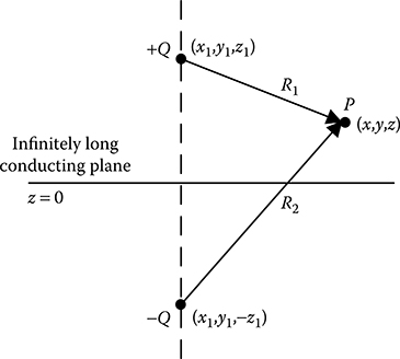
FIGURE 9.1
Point charge near an infinitely long conducting plane.

Considering the conducting plane to be the x–y plane, the problem is to find a solution for electric field in the region z > 0. This solution can be obtained by solving Laplace’s equation with the following conditions:

The solution ϕ(x,y,z) will be valid at every point for z > 0 except the location of the point charge.
The potential at all the points on the conducting plane is zero, that is, ϕ(x,y,0) = 0.
The potential approaches zero as the distance from the charge approaches infinity.

It is not easy to find a solution to Laplace’s equation that satisfies all the above conditions.

The problem can also be viewed from another angle. The positive polarity point charge at z = z₁ will induce negative polarity charges on the surface of the conducting plane. Say, the induced surface charge density is −σ_s. Then the electric field at any point in the region z > 0 will be due to the point charge and the induced surface charges. But the difficulty is that σ_s needs to be determined using the boundary condition ϕ(x,y,0) = 0, before the solution to electric field in the region z > 0 could be obtained. Furthermore, the evaluation of the surface integral to obtain the field due to the induced charges is not an easy task. From all these considerations, taking the image of the point charge with respect to the infinitely long conducting plane to replace the plane by the image charge is an easy and practical methodology.

The electric potential at a distance r from a point charge is given by Q/(4πε₀r). Considering the spherical symmetry of the field due to a point charge, it may be seen that the electric field due to a point charge is dependent only on r-coordinate in spherical coordinate system and is independent of θ and ϕ coordinates. Hence, this electric potential satisfies Laplace’s equation in spherical coordinates as follows:

${\vec{\nabla}}^{2} ϕ = \frac{1}{r^{2}} \frac{\partial}{\partial r} (r^{2} \frac{\partial ϕ}{\partial r}) = \frac{1}{r^{2}} \frac{\partial}{\partial r} (r^{2} \times - \frac{Q}{4 π ε_{0} r^{2}}) = \frac{1}{r^{2}} \frac{\partial}{\partial r} (- \frac{Q}{4 π ε_{0}}) = 0$

Consider that the infinitely long conducting plane is replaced by a fictitious discrete point charge of magnitude Q₁ located at (x₁,y₁,−z₂). Because the field due to a point charge satisfies Laplace’s equation, the field due to the real point charge and the image point charge will also satisfy Laplace’s equation at all points for z > 0 except at the location of the real point charge.

Therefore, the electric potential at any point P(x,y,z) will be given by

$ϕ_{P} = \frac{Q}{4 π ε_{0} R_{1}} + \frac{Q_{1}}{4 π ε_{0} R_{2}} (9.1)$

where:

$\begin{matrix} R_{1} = [(x - x_{1})^{2} + (y - y_{1})^{2} + (z - z_{1})^{2}]^{1 / 2} \\ and R_{2} = [(x - x_{1})^{2} + (y - y_{1})^{2} + (z + z_{2})^{2}]^{1 / 2} \end{matrix}$

From Equation 9.1, it is evident that the potential at a very large distance from the point charge Q will be zero.

Therefore, two of the above-mentioned three conditions are satisfied by Equation 9.1. In order to satisfy the third condition, ϕ_P at any point on the conducting plane has to be zero. From Equation 9.1, it is obvious that the polarity of Q₁ has to be negative to satisfy this condition. Furthermore, the following has to be satisfied at all the points on the conducting plane

$\frac{Q}{R_{1}} = \frac{Q_{1}}{R_{2}} (9.2)$

The best solution for Equation 9.2 is obtained when the magnitude of the image charge (Q₁) is equal to the magnitude of the real charge (Q) and location of the image charge is such that the magnitudes of R₁ and R₂ are equal at all the points on the conducting plane. From the expressions of R₁ and R₂, it is clear that for z = 0, R₁ will be equal to R₂ if z₁ = z₂. Therefore, the third condition will also be satisfied if Q₁ = −Q and the location of the image charge is at (x₁,y₁,−z₁).

Thus, the combination of the real charge Q located at (x₁,y₁,z₁) and the image charge −Q located at (x₁,y₁,−z₁) satisfies all the three conditions stated above. Hence, the electric field in the region z > 0 due to the real point charge +Q and the infinitely long conducting plane will be the same as that due to +Q and −Q located as mentioned above.

Therefore, the electric potential at any point P(x,y,z) for z > 0 will be given by

$ϕ_{P} = \frac{Q}{4 π ε_{0}} (\frac{1}{R_{1}} - \frac{1}{R_{2}}) (9.3)$

where:

$\begin{matrix} R_{1} = [(x - x_{1})^{2} + (y - y_{1})^{2} + (z - z_{1})^{2}]^{1 / 2} \\ and R_{2} = [(x - x_{1})^{2} + (y - y_{1})^{2} + (z + z_{2})^{2}]^{1 / 2} \end{matrix}$

In Cartesian coordinates, electric field intensity at any point P(x,y,z) for z > 0 will be given by

${\vec{E}}_{P} = - \frac{\partial ϕ_{P}}{\partial x} \hat{i} - \frac{\partial ϕ_{P}}{\partial y} \hat{j} - \frac{\partial ϕ_{P}}{\partial z} \hat{k} (9.4)$

where:

$\begin{matrix} E_{x P} = - \frac{\partial ϕ_{P}}{\partial x} = \frac{Q}{4 π ε_{0}} (\frac{x - x_{1}}{R_{1}^{3}} - \frac{x - x_{1}}{R_{2}^{3}}) \\ E_{yP} = - \frac{\partial ϕ_{P}}{\partial x} = \frac{Q}{4 π ε_{0}} (\frac{y - y_{1}}{R_{1}^{3}} - \frac{y - y_{1}}{R_{2}^{3}}) \\ E_{z P} = - \frac{\partial ϕ_{P}}{\partial z} = \frac{Q}{4 π ε_{0}} (\frac{z - z_{1}}{R_{1}^{3}} - \frac{z + z_{1}}{R_{2}^{3}}) \end{matrix}$

For any point very near to the conducting plane, that is, z → 0, R₁ ≈ R₂. Hence, E_xP and E_yP will be zero. Thus,

$\begin{matrix} \lim_{z \to 0} {\vec{E}}_{z P} = \frac{σ_{s}}{ε_{0}} \hat{k} = \frac{- Q z_{1}}{2 π ε_{0} [(x - x_{1})^{2} + (y - y_{1})^{2} + z_{1}^{2}]^{3 / 2}} \hat{k} \\ or σ_{s} = \frac{- Q z_{1}}{2 π [(x - x_{1})^{2} + (y - y_{1})^{2} + z_{1}^{2}]^{3 / 2}} \end{matrix} (9.5)$

Equation 9.5 gives the negative surface charge density induced on the conducting plane by the positive polarity real point charge.

This problem can also be viewed from a different perspective. The field due to the real point charge and the image point charge is the same as that due to a spatially extended electric dipole. Considering spherical coordinates and assuming that the electric dipole to be oriented along the axis of symmetry, as shown in Figure 9.2, electric potential and electric field intensity can be expressed in spherical coordinates.

With reference to Figure 9.2,

$\begin{matrix} r_{1} = (r^{2} + h^{2} - 2 r h \cos θ)^{1 / 2} and \\ r_{2} = [r^{2} + h^{2} - 2 r h \cos (π - θ)]^{1 / 2} = (r^{2} + h^{2} + 2 r h \cos θ)^{1 / 2} \end{matrix} (9.6)$

Then,

$ϕ_{P} = \frac{Q}{4 π ε_{0}} [\frac{1}{(r^{2} + h^{2} - 2 r h \cos θ)^{1 / 2}} - \frac{1}{(r^{2} + h^{2} + 2 r h \cos θ)^{1 / 2}}] (9.7)$

${\vec{E}}_{P} = - \frac{\partial ϕ_{P}}{\partial r} {\hat{u}}_{r} - \frac{1}{r} \frac{\partial ϕ_{P}}{\partial θ} {\hat{u}}_{θ} - \frac{l}{r \sin θ} \frac{\partial ϕ_{P}}{\partial ϕ} {\hat{u}}_{ϕ} (9.8)$

where:

$E_{r P} = - \frac{\partial ϕ_{P}}{\partial r} = - \frac{Q}{4 π ε_{0}} (\frac{r - h \cos θ}{r_{1}^{3}} - \frac{r + h \cos θ}{r_{2}^{3}})$

Images

FIGURE 9.2
Electric dipole formed by the real and image charges.

$\begin{matrix} E_{θ P} = - \frac{1}{r} \frac{\partial ϕ_{P}}{\partial θ} = \frac{Q h \sin θ}{4 π ε_{0}} (\frac{1}{r_{1}^{3}} - \frac{1}{r_{2}^{3}}) \\ and {\vec{E}}_{ϕ P} = - \frac{l}{r \sin θ} \frac{\partial ϕ_{P}}{\partial ϕ} = 0 . \end{matrix}$

Equations 9.7 and 9.8 are the expressions for the electric field due to an electric dipole of dipole moment $\vec{M} = 2 Q h \hat{k}$ , as shown in Figure 9.2.

However, it is to be noted here that the solution obtained with the help of image charge is valid only for the region z > 0 as for z < 0 the region is below an infinitely long conducting plane whose potential is zero and hence for z < 0, the electric field is zero. The image charge does not exist in reality as it is a fictitious charge.

9.2.1 Point Charge between Two Conducting Planes

Consider two conducting planes making an angle θ between them, as shown in Figure 9.3a, such that 2π is integer multiple of θ. Consider also that the potential of the conducting planes is zero and there is a point charge +Q in the wedge-shaped space between the two conducting planes. A direct solution of Laplace’s equation subject to boundary condition of zero electric potential on the conducting planes would be quite difficult. However, this problem could be solved by introducing image charges considering the conducting planes as mirrors. Then n number of image charges are introduced at each location where the conducting planes acting as mirrors would form images of the real point charge, where n = (2π/θ) − 1. Such images are shown in Figure 9.3a, where θ = 60°. The pair of charges +Q and −Q separated by 2h₁, 2h₂, 2h₃, 2h₄, 2h₅ and 2h₆ will make the potential zero for Plane A, Plane B, Plane A, Plane B, Plane B and Plane A, respectively. The solution then will be unique as the boundary conditions are satisfied. But this solution will be valid only in the wedge-shaped space between the two conducting planes. Another case of two conducting planes making an angle θ = 90° is shown in Figure 9.3b.

Images

FIGURE 9.3
Point charge between two conducting planes: (a) between two planes making an angle θ and (b) between two perpendicular planes.

9.3 Image of a Point Charge with Respect to a Grounded Conducting Sphere

Image of a charge is not necessarily to be taken with respect to infinitely long plane only. It can also be taken with respect to curved surfaces such as sphere, cylinder and so on. To elaborate this issue, consider a point charge +Q located at distance d from the centre (O) of the sphere of radius a (a < d), as shown in Figure 9.4. Consider also that the electric potential of the sphere is zero. The field due to the point charge and the grounded sphere in the region outside the sphere could be determined by replacing the grounded sphere by an image point charge. From the symmetry of the system, it is evident that the image charge q will be of negative polarity and will be located inside the sphere on the line joining the centre of the sphere and the point charge, as shown in Figure 9.4. However, in this case, the magnitude of q will not be equal to Q because such a pair of charges will not result into a zero-potential spherical surface of radius a as required by the boundary condition.

Images

FIGURE 9.4
Point charge near a grounded sphere.

Consider that the image charge is located at a distance s from the centre of the sphere, as shown in Figure 9.4. Now the problem is to determine the magnitude as well as the location of the image charge that satisfies the zero-potential boundary condition for the spherical surface. With reference to Figure 9.4, the potential at the point P due to the point charge and its image is given by

$ϕ_{P} = \frac{1}{4 π ε_{0}} (\frac{Q}{r_{1}} - \frac{Q}{r_{2}}) (9.9)$

Imposition of the boundary condition ϕ_P = 0 leads to

$\frac{q}{Q} = \frac{r_{2}}{r_{1}} = α (9.10)$

If α is kept constant, then r₁/r₁ = constant is the equation of a sphere. Hence, the problem now is to find the constant α.

For the point 1, as shown in Figure 9.4, α = r₂/r₁ = (a – s)/(d – a) and for the point 2, as shown in Figure 9.4, α = r₂/r₁ = (a + s)/(d + a).

$Therefore, α = \frac{r_{2}}{r_{1}} = \frac{a - s}{d - a} = \frac{a + s}{d + a} = \frac{a}{d} = \frac{s}{a} (by componendo - dividendo) (9.11)$

Because the radius of the sphere and the location of the point charge are known, the constant α can be computed from the ratio of a and d, as given by Equation 9.11.

Therefore, the magnitude of the image charge is given by

$q = \frac{a}{d} Q (9.12)$

and the location of the image charge is given by

$s = \frac{a^{2}}{d} (9.13)$

Considering the line joining the point charge and its image passing through the centre of the sphere to be along the z-axis and the centre of the sphere to be the origin, as shown in Figure 9.4, and also taking into account the spherical symmetry of the configuration, the field can be expressed in spherical coordinates as follows.

With reference to the point P of Figure 9.4,

$r_{1} = | {\vec{r}}_{P} - r_{+ Q} | = (a^{2} + d^{2} - 2 a d \cos θ)^{1 / 2}$

where:

θ is the angle between a and d at P

$r_{2} = | {\vec{r}}_{P} - r_{- q} | = (a^{2} + s^{2} - 2 a s \cos θ)^{1 / 2}$

Similarly, for any point in the field region for which r is the distance of the point from the origin, that is, the centre of the sphere, and θ is the angle between r and d

$\begin{matrix} r_{1} = | \vec{r} - r_{+Q} | = (r^{2} + d^{2} - 2 r d \cos θ)^{1 / 2} and \\ r_{2} & = | \vec{r} - {\vec{r}}_{- q} | = (r^{2} + s^{2} - 2 r s \cos θ)^{1 / 2} = (r^{2} + \frac{a^{4}}{d^{2}} - 2 r \frac{a^{2}}{d} \cos θ)^{1 / 2} \\ = {(\frac{r^{2} d^{2} + a^{4} - 2 r d a^{2} \cos θ}{d^{2}})}^{1 / 2} \end{matrix}$

Therefore, the electric potential at any point due to the point charge and its image is given by

$ϕ (r, θ) = \frac{Q}{4 π ε_{0}} [\frac{1}{(r^{2} + d^{2} - 2 r d \cos θ)^{1 / 2}} - \frac{a}{(r^{2} d^{2} + a^{4} - 2 r d a^{2} \cos θ)^{1 / 2}}] (9.14)$

Therefore,

${\vec{E}}_{_{r}} (a, θ) = - \frac{\partial ϕ (r, θ)}{\partial r} |_{r = a} = - \frac{Q}{4 π ε_{0} a} \frac{d^{2} - a^{2}}{(a^{2} + d^{2} - 2 a d \cos θ)^{3 / 2}} (9.15)$

Now, r-component of electric field intensity is the normal component on the sphere surface. Therefore, assuming the induced surface charge density on the sphere surface to be σ_s, the normal component of electric field intensity is equal to σ_s/ε₀ just off the sphere surface. Equating this expression with the one given by Equation 9.15, the induced surface charge density on the grounded sphere surface is given by

$σ_{s} = \frac{Q}{4 π a} \frac{d^{2} - a^{2}}{(a^{2} + d^{2} - 2 a d \cos θ)^{3 / 2}} (9.16)$

9.3.1 Method of Successive Images

Sphere-gap arrangements are very commonly used in high-voltage system for voltage measurement. As shown in Figure 9.5, in this arrangement, two spheres of identical radius (a) are separated by a specific distance s, where one sphere is charged while the other is earthed. The field within the sphere gap due to the two spheres could be analyzed with the help of image charges, as described in Section 9.3. The live sphere of potential V is at first replaced by a charge of magnitude Q_A = 4πε₀aV located at the centre of the live sphere. Then to keep the potential of the grounded sphere at zero, −q₁ is introduced within the grounded sphere, which is the image of Q_A, as shown in Figure 9.5. The magnitude and location of q₁ are given by

$q_{1} = \frac{a}{d} Q_{A} and s_{1} = \frac{a^{2}}{d} (9.17)$

Images

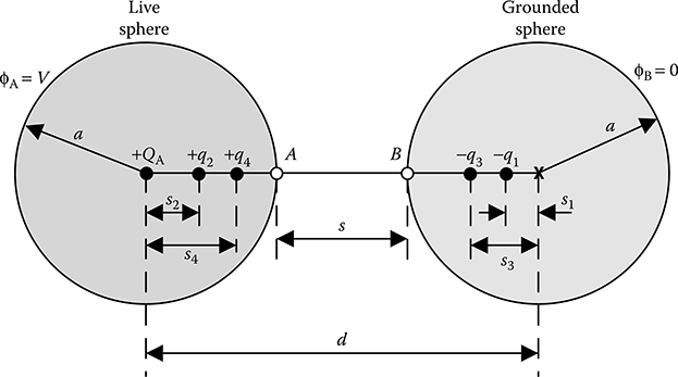
FIGURE 9.5
Method of successive imaging as applied to sphere-gap arrangement.

But the introduction of −q₁ will make the potential of live sphere different from V. Therefore, to keep the potential of live sphere equal to V, +q₂, which is the image of −q₁, is introduced within the live sphere such that the potential of live sphere due to +q₂ and −q₁ will be zero. As a result, the potential of live sphere due to +Q_A, −q₁ and +q₂ will be again V. The magnitude and location of q₂ are given by

$q_{2} = \frac{a}{d - s_{1}} q_{1} = \frac{a^{2}}{d (d - s_{1})} Q_{A} and s_{1} = \frac{a^{2}}{d - s_{1}} (9.18)$

But the introduction of +q₂ will make the potential of grounded sphere different from zero. Therefore, −q₃ is introduced within the grounded sphere as the image of +q₂ to make the potential of the grounded sphere equal to zero. Further, the introduction of −q₃ warrants introduction of +q₄ within the live sphere and so on. In this way, there will be an infinite series of charges within the two spheres: positive charges such as +Q_A, +q₂ and +q₄ within the live sphere and negative charges such as −q₁ and −q₃ within the grounded sphere. This method of taking successive image charges within the two spheres is known as the method of successive imaging. It may be seen from Equations 9.17 and 9.18 that each successive image charge is smaller in magnitude and gradually shifts towards the surface of the sphere within which it is located. In all practicality, it is adequate to take the first few images within the two spheres to achieve reasonably good accuracy in the computation of electric field. In the sphere-gap arrangement, maximum value of electric field intensity occurs at the so-called sparking tips of the spheres, namely, points A and B, as shown in Figure 9.5. This maximum electric field intensity can be obtained as

$E_{\max} = \frac{V}{s} [\frac{(s / a + 1) + \sqrt{(s / a + 1)^{2} + 8}}{4}] (9.19)$

As discussed in Section 4.7, E_av = V/s

Therefore, field factor (f) for sphere-gap arrangement is as follows:

$\frac{E_{\max}}{E_{a v}} = [\frac{(s / a + 1) + \sqrt{(s / a + 1)^{2} + 8}}{4}] (9.20)$

Variation of field factor (f) with gap distance (s) in the case of sphere-gap arrangement is presented in Table 9.1. It may be seen from Table 9.1 that the deviation from a uniform field (f = 1) for s/a = 0.2 is 6.8%, whereas that for s/a = 1.0 is 36.6%. Accuracy of voltage measurement by the sphere gap depends significantly on the degree of field non-uniformity between the two spheres. Hence, it is recommended in practice that the gap distance should not be made more than the radius of the spheres.

TABLE 9.1
Variation of Field Factor with Gap Distance for Sphere Gap

Images

PROBLEM 9.1

Two spheres of 25 cm diameter have a gap distance of 2.5 cm between them. Determine the breakdown voltage of the sphere gap in air at standard temperature and pressure (STP).

Solution:

Given s = 2.5 cm and a = (25/2) = 12.5 cm.

Therefore, s/a = 2.5/12.5 = 0.2. Correspondingly, field factor (f) = 1.068.
E_max corresponding to breakdown of air at STP is 30 kV_p/cm.

Therefore,

$E_{a v} = \frac{E_{\max}}{f} = \frac{30}{1.0 68} = 28.0 9 k V_{p} / c m$

But,

$E_{a v} = \frac{V}{s}$

Hence,

$\frac{V}{2.5} = 28.0 9, or, V = 70.22 {kV}_{P}$

9.3.2 Conducting Sphere in a Uniform Field

The problem of a conducting sphere placed in a uniform external field can be solved with the help of image charges, as discussed in Section 9.3. As shown in Figure 9.6, consider that the centre of the sphere is located at the origin O. The uniform external field is assumed to be created by two point charges −Q and +Q located at (0,0,d) and (0,0,−d), respectively. The field due to these two charges at the origin is given by

$E_{0} = \frac{2 Q}{4 π ε_{0} d^{2}} {\hat{U}}_{z} (9.21)$

If d is very large compared to the radius of the sphere a, then the field intensity will have approximately the value given by Equation 9.21 in the proximity of the sphere. The difference becomes negligibly small when (d/a) → ∞. Then the configuration is equivalent to a conducting sphere in a uniform external field.

Images

FIGURE 9.6
Conducting sphere in a uniform external field.

To solve this problem, two image charges +q and −q are placed at (0,0,+s) and (0,0,−s), respectively, where s = (a²/d). This will make the potential of the sphere to be zero. However, the sphere can also be considered as isolated, that is, electrically not connected to any other body, because the total image charge within the sphere is zero.

Then the potential at any point in the vicinity but outside the sphere can be written with the help of Equation 9.14 as follows:

$ϕ (r, θ) = \frac{Q}{4 π ε_{0}} [\begin{matrix} \frac{1}{(r^{2} + d^{2} + 2 r d c o s θ)^{1 / 2}} - \frac{a}{(r^{2} d^{2} + a^{4} + 2 r d a^{2} c o s θ)^{1 / 2}} \\ - \frac{1}{(r^{2} + d^{2} - 2 r d c o s θ)^{1 / 2}} + \frac{a}{(r^{2} d^{2} + a^{4} - 2 r d a^{2} c o s θ)^{1 / 2}} \end{matrix}] (9.22)$

The potential in the limiting condition of d → ∞,

$ϕ (r, θ) \approx - \frac{2 Q r \cos θ}{4 π ε_{0} d^{2}} (1 - \frac{a^{3}}{r^{3}}) \approx - E_{0} r \cos θ (1 - \frac{a^{3}}{r^{3}}) (9.23)$

In Equation 9.23, the first term −E₀r cos θ = −E₀z is the potential due to the uniform external field and the second term is the potential due to the induced charge density on the surface of the sphere.

9.4 Image of an Infinitely Long Line Charge with Respect to an Infinitely Long Conducting Plane

Consider an infinitely long line charge of positive polarity and uniform line charge density +λ_l is located parallel to an infinitely long conducting plane present at y = 0 and is at a height y₁ from the plane, as shown in Figure 9.7, such that the location of the line charge is given by (x₁,y₁). The configuration as shown in Figure 9.7 depicts the view on the cross-sectional plane perpendicular to the length of the charge and the plane. As discussed in Section 9.2, the practical example of such a plane is the earth surface having zero potential. The problem is, therefore, a two-dimensional one in Cartesian coordinates, where the field varies only on the x–y plane, that is, the cross-sectional plane.

Therefore, the problem is to find a solution for electric field in the region y > 0. As discussed in Section 9.2, this solution can be obtained by solving Laplace’s equation with the following conditions:

The solution ϕ(x,y) will be valid at every point for y > 0 except the location of the line charge.
The potential at all the points on the conducting plane is zero, that is, ϕ(x,0) = 0.
The potential approaches zero as the distance from the charge approaches infinity.

Images

FIGURE 9.7
Infinitely long line charge near an infinitely long conducting plane.

The electric potential at a distance r from an infinitely long line charge is given by Q/(2πε₀)ln(R/r), where R → ∞. Considering the cylindrical symmetry of the field due to an infinitely long line charge, it may be seen that the electric field due to an infinitely long line charge is dependent only on r-coordinate in cylindrical coordinate system and is independent of θ and z coordinates. Hence, this electric potential satisfies Laplace’s equation in cylindrical coordinates as follows:

${\vec{\nabla}}^{2} ϕ = \frac{1}{r} \frac{\partial}{\partial r} (r \frac{\partial ϕ}{\partial r}) = \frac{1}{r} \frac{\partial}{\partial r} (r \times - \frac{Q}{2 π ε_{0} r}) = \frac{1}{r} \frac{\partial}{\partial r} (- \frac{Q}{2 π ε_{0}}) = 0 (9.24)$

Similar to the discussion of Section 9.2, the infinitely long conducting plane is replaced by a fictitious line charge of the uniform line charge density −λ_l located at (x₁,−y₁), which is the image of the real line charge. Because the field due to an infinitely long line charge satisfies Laplace’s equation, the field due to the real line charge and the image line charge will also satisfy Laplace’s equation at all points for y > 0 except at the location of the real line charge.

Therefore, the electric potential at any point P(x,y) will be given by

$ϕ_{P} = \frac{λ_{l}}{2 π ε_{0}} \ln \frac{R_{2}}{R_{1}} (9.25)$

where:

$\begin{matrix} R_{1} = [(x - x_{1})^{2} + (y - y_{1})^{2}]^{1 / 2} \\ and R_{2} = [(x - x_{1})^{2} + (y + y_{1})^{2}]^{1 / 2} \end{matrix}$

From Equation 9.25, it is evident that the potential at a very large distance from the line charge will be zero and also that the potential at all the points on the conducting plane at y = 0 will be zero, because at every point on the plane R₁ = R₂.

In Cartesian coordinates for a two-dimensional system, the electric field intensity at any point P(x,y) for y > 0 will be given by

${\vec{E}}_{P} = - \frac{\partial ϕ_{P}}{\partial x} \hat{i} - \frac{\partial ϕ_{P}}{\partial y} \hat{j} (9.26)$

where:

$\begin{array}{l} E_{x P} = - \frac{\partial ϕ_{P}}{\partial x} = \frac{Q}{2 π ε_{0}} (\frac{x - x_{1}}{R_{1}^{2}} - \frac{x - x_{1}}{R_{2}^{2}}) \\ E_{y P} = - \frac{\partial ϕ_{P}}{\partial y} = \frac{Q}{2 π ε_{0}} (\frac{y - y_{1}}{R_{1}^{2}} - \frac{y + y_{1}}{R_{2}^{2}}) \end{array}$

For any point very near to the conducting plane, that is, y → 0, R₁ ≈ R₂. Hence, E_xP will be zero. Thus

$\begin{matrix} \lim_{y \to 0} {\vec{E}}_{y P} = \frac{σ_{s}}{ε_{0}} \hat{k} = \frac{- Q y_{1}}{π ε_{0} [(x - x_{1})^{2} + y_{1}^{2}]^{3 / 2}} \hat{k} \\ o r, σ_{s} = \frac{- Q y_{1}}{π [(x - x_{1})^{2} + y_{1}^{2}]^{3 / 2}} \end{matrix} (9.27)$

Equation 9.27 gives the negative surface charge density induced on the conducting plane by the positive polarity real line charge.

From Equation 9.25, an expression for the equipotential surface can be obtained as follows:

$\frac{R_{2}}{R_{1}} = α$

where:

α is a constant

$\begin{matrix} or, (x - x_{1})^{2} + (y + y_{1})^{2} = α^{2} [(x - x_{1})^{2} + (y - y_{1})^{2}] \\ or, (x - x_{1})^{2} + {(y - y_{1} \frac{α^{2} + 1}{α^{2} - 1})}^{2} = {(\frac{2 α y_{1}}{α^{2} - 1})}^{2} \end{matrix} (9.28)$

Equation 9.28 shows that the equipotentials are circles of radius |(2αy₁)/(α² – 1)| having centre at x₁, (α² + 1)/(α² – 1)y₁ on the cross-sectional plane. For the infinite conducting plane of zero potential α = 1. For equipotentials above the infinite conducting plane α > 1 and those below the infinite conducting plane α < 1. In physical terms, the equipotentials are circular cylinders with axes parallel to the two line charges, as shown in Figure 9.8. As α increases the radius of the cylinder increases and the axis of the cylinder shifts further away from the line charge.

The equipotentials below the conducting planes do not have any physical meaning as the electric field is zero below the infinitely long conducting plane. But the equipotentials, as shown in Figure 9.8, give an important idea that two parallel cylinders having electric potentials +V and −V could be replaced by two infinitely long line charges. However, the line charges will not be located at the axes of the cylinders.

Images

FIGURE 9.8
Equipotentials for an infinitely long charge and its image with respect to an infinitely long conducting plane.

9.5 Two Infinitely Long Parallel Cylinders

Electric field due to two parallel cylindrical transmission line conductors is the same as the field due to two infinitely long parallel cylinders. The cross-sectional view of the arrangement is shown in Figure 9.9. Electric field for this arrangement is two dimensional in Cartesian coordinates, because the field does not vary along the z-axis, which is along the length of the cylinders. Electric field varies only on the cross-sectional plane, which is taken as the x–y plane. As discussed in Section 9.4, these two parallel cylinders having potential +V and −V could be replaced by two infinitely long line charges of the uniform line charge density +λ_l and −λ_l located within the respective cylinders, as shown in Figure 9.9. These two line charges together will create two cylindrical equipotential surfaces of radius a having the specified potentials +V and −V. The charges will be located at a distance s from the axis of the respective cylinders. Therefore, the problem is to find the location of these charges.

Images

FIGURE 9.9
Two infinitely long parallel cylinders replaced by two infinitely long line charges.

With reference to Figure 9.9, the potential of the point P on the surface of the cylinder is

$ϕ_{P} = \frac{λ_{1}}{2 π ε_{0}} \ln \frac{R_{2}}{R_{1}}$

For the cylinder surface to be equipotential the ratio of R₂ to R₁ must be constant.

Considering the point 1 on the cylinder surface, as shown in Figure 9.9,

$ϕ_{1} = \frac{λ_{1}}{2 π ε_{0}} \ln \frac{d + a - s}{a + s} (9.29)$

and for the point 2 on the cylinder surface, as shown in Figure 9.9,

$ϕ_{2} = \frac{λ_{1}}{2 π ε_{0}} \ln \frac{d - a - s}{a - s} (9.30)$

But, ϕ₁ = ϕ₂. Hence, (d + a – s)/(a + s) = (d – a – s)/(a – s) = (d – s)/(a = a/s (by componendo–dividendo)

Therefore,

$\begin{matrix} s^{2} - s d + a^{2} = 0 \\ or, s = \frac{d}{2} \pm \frac{\sqrt{d^{2} - 4 a^{2}}}{2} \end{matrix} (9.31)$

In the solution of s as given by Equation 9.31, the additive expression has to be neglected, because in that case the image charge will be located outside the cylinder. Therefore,

$s = \frac{d}{2} - \frac{\sqrt{d^{2} - 4 a^{2}}}{2} (9.32)$

For transmission lines, d ≫ a and hence s ≈ 0, that is, the line charges are placed on the axes of the two cylinders.

Now, the potential at the point 2 on the cylinder surface, as shown in Figure 9.9, is +V. Hence,

$\begin{matrix} ϕ_{2} = \frac{λ_{1}}{2 π ε_{0}} \ln \frac{d - a - s}{a - s} = V \\ or, λ_{1} = \frac{2 π ε_{0} V}{\ln [(d - a - s) / (a - s)]} \end{matrix} (9.33)$

Equation 9.33 gives the magnitude of the uniform line charge density.

In the arrangement shown in Figure 9.9, maximum electric field intensity (E_max) occurs at the point 2, which is given by

$E_{\max} = \frac{λ_{1}}{2 π ε_{0}} (\frac{1}{a - s} + \frac{1}{d - a - s}) = \frac{V}{\ln [(d - a - s) / (a - s)]} (\frac{1}{a - s} + \frac{1}{d - a - s}) (9.34)$

Right-hand side (RHS) of Equation 9.34 is in terms of the physical dimensions of the arrangement and the electric potential of the cylinders and hence can be computed in a straightforward manner.

Again, for the physical arrangement of Figure 9.9, E_av = 2V/(d – 2a).

Therefore, field factor

$(f) = \frac{E_{max}}{E_{av}} = \frac{(d - 2 a)}{2 \ln [(d - a - s) / (a - s)]} (\frac{1}{a - s} + \frac{1}{d - a - s}) (9.35)$

Putting the value of s from Equation 9.32 in Equation 9.35 and simplifying it may be written that

$f = \frac{\sqrt{(d / 2 a)^{2} - 1}}{\ln [(d / 2 a) + \sqrt{(d / 2 a)^{2} - 1}]} (9.36)$

For transmission lines, Equation 9.36 is often modified by putting d = X + 2a, which yields

$f = \frac{\sqrt{(X / a)^{2} + 4 (X / a)}}{2 \ln [(X / 2 a) + 1 + (1 / 2) \sqrt{(X / a)^{2} + 4 (X / a)}]} (9.37)$

Equation 9.37 represents the field factor as a function of the ratio of the gap distance between the two transmission line conductors (X) and the radius of the conductors (a).

For high-voltage transmission lines, d ≫ a. As a result the field factor as given by Equation 9.36 reduces to

$\begin{matrix} f = \frac{d}{2 a \ln (d / a)} \\ and E_{a v} = \frac{2 V}{d - 2 a} \approx \frac{2 V}{d} \end{matrix} (9.38)$

Hence,

$E_{\max} = E_{a v} \times f = \frac{2 V}{d} \times \frac{d}{2 a \ln (d / a)} = \frac{V}{a \ln (d / a)} (9.39)$

Capacitance per unit length between the two parallel cylinders can be obtained from Equations 9.32 and 9.33 as follows:

$C = \frac{λ_{1}}{2 V} = \frac{π ε_{0}}{\ln [(d - a - s) / (a - s)]} = \frac{π ε_{0}}{\ln [(d / 2 a) + \sqrt{(d / 2 a)^{2} - 1}} (9.40)$

Because $\ln (x + \sqrt{x^{2} - 1}) = cos h^{- 1} x$ , for x > 1 Equation 9.40 can be written as follows:

$C = \frac{π ε_{0}}{\cos h^{- 1} (d / 2 a)} (9.41)$

PROBLEM 9.2

A long conductor of negligible radius is at a height 5 m from the earth surface and is parallel to it. It has a uniform line charge density of +1 nC/m. Find the electric potential and field intensity at a point 3 m below the line.

Solution:

The arrangement of the problem is shown in Figure 9.10. Because the conductor is considered to have negligible radius, the line charge is located on the axis of the conductor.

With reference to Equation 9.25, λ_l = 1 nC/m, R₁ = 3 m and R₂ = 7 m.

Therefore,

$ϕ_{P} = \frac{1 0^{- 9}}{2 π \times 8.8 54 \times 1 0^{- 12}} \ln \frac{7}{3} = 15.2 3 V$

Electric field intensity components at the point P are obtained from Equation 9.26 as follows:

$\begin{matrix} E_{x P} = 0 \\ E_{y P} = \frac{1 0^{- 9}}{2 π \times 8.8 54 \times 1 0^{- 12}} (\frac{2 - 5}{3^{2}} - \frac{2 + 5}{7^{2}}) = - 8.5 6 V / m . \end{matrix}$

Images

FIGURE 9.10
Pertaining to Problem 9.2.

PROBLEM 9.3

Determine the breakdown voltage in air at standard temperature and pressure (STP) of a 20 cm diameter cylindrical electrode placed horizontally with its axis 20 cm above the earth surface.

Solution:

The arrangement of the problem is shown in Figure 9.11.

With reference to Equation 9.36 d = 40 cm and a = 10 cm. Hence, (d/2a) = 2.

Therefore,

$f = \frac{\sqrt{2^{2} - 1}}{\ln (2 + \sqrt{2^{2} - 1})} = 1.3 15$

Images

FIGURE 9.11
Pertaining to Problem 9.3.

E_max corresponding to breakdown of air at STP is 30 kV_p/cm.

Therefore,

$E_{a v} = \frac{E_{\max}}{f} = \frac{30}{1.3 15} = 22.8 1 k V_{p} / c m$

But,

E_av = (2V)/(d – 2a)

Hence,

2V/20 = 22.81, or, V = 228.1 kV_p

9.6 Salient Features of Method of Images

Image charges are always located outside the region where the field is to be determined.
Depending on the type of problem, the magnitude of image charge may or may not be the same as that of the physical charge.
Depending on the type of problem, image charges may or may not be of polarity opposite to that of the physical charge.
In the image charge system, electric field is finite on both sides of the imaging surface. But in the physical system, electric field is non-zero and finite only on one side of the imaging surface. Because energy in electric field is proportional to volume integral of E², the electrostatic energy in the physical charge system is half of the electrostatic energy of the image charge system.

Objective Type Questions

1. Image charge should always be placed

a. At a finite distance within the region where field is to be computed

b. At a finite distance outside the region where field is to be computed

c. On the imaging surface

d. At infnity

2. Image of a charge can be taken with respect to

a. A finitely long conducting plane

b. An infinitely long conducting plane

c. A curved surface such as cylinder or sphere

d. Both (b) and (c)

3. Electrostatic energy in the physical charge system only is

a. Square of the electrostatic energy of the image charge system

b. Double the electrostatic energy of the image charge system

c. Equal to the electrostatic energy of the image charge system

d. Half of the electrostatic energy of the image charge system

4. A point charge is placed in the wedge-shaped space between two grounded conducting planes making an angle 60° between them. Then the number of image charges will be

a. 2

b. 4

c. 5

d. 6

5. A point charge is placed in the space between two perpendicular conducting planes. Then

a. All the three image charges will be of negative polarity

b. Two image charges will be of negative polarity

c. One image charge will be of negative polarity

d. None of the image charges will be of negative polarity

6. Two long parallel cylinders of same radius with a specific separation distance can be replaced by two infinite line charges where

a. Both the charges are located at the axes of the cylinders

b. One charge is located at the axis of one cylinder, whereas the other is located away from the axis of the other cylinder

c. Both the charges are located away from the axes of the cylinders

d. Both the charges are located on the surface of the cylinders

7. Two identical spheres with a specific gap distance can be replaced by

a. Two point charges located at the centres of the two spheres

b. Two point charges located away from the centres of the two spheres

c. Two point charges located on the surface of the two spheres

d. Infinite number of point charges located within the two spheres

8. Method of successive images is used in the case of

a. Two identical spheres

b. A point charge near a grounded sphere

c. Two long parallel cylinders

d. A line charge near a long parallel grounded cylinder

9. Equipotentials due to two infinitely long parallel line charges will be

a. Infinitely long cylinders of circular cross section

b. Finite length cylinders of circular cross section

c. Infinitely long cylinders of elliptical cross section

d. Finite length cylinders of elliptical cross section

10. A point charge of magnitude Q is placed at a distance d from the centre of a grounded sphere of radius a (a < d). Then the magnitude of the image charge to replace the grounded sphere will be

a. (a/d)Q

b. (a/d²)Q

c. (a²/d)Q

d. (a²/d²)Q

Answers:

1) b;

2) d;

3) d;

4) c;

5) b;

6) c;

7) d;

8) a;

9) a;

10) a

..................Content has been hidden....................

You can't read the all page of ebook, please click here login for view all page.

Table of Contents for 9. Method of Images

Create new playlist

Sign In

Sign Up

PROBLEM 9.1

PROBLEM 9.2

PROBLEM 9.3

Answers:

Table of Contents for
9. Method of Images