1. Fundamentals of Electric Field

Search in book...
Toggle Font Controls
Create new playlist

Name your new playlist

Playlist description (optional)
Sign In

Email address

Password

Forgot Password?

or

Continue with Facebook

Continue with Google
Sign Up

Full Name

Email address

Confirm Email Address

Password

or

Continue with Facebook

Continue with Google

ABSTRACT Leaving aside nuclear interactions, there are two non-contact forces that act at a distance, namely, gravitational and electric forces. Gravitational force is dominant at large distances whereas electric forces are dominant at shorter distances. The root cause of electric forces is electric charge. The effect of electric charge is spread over the entire space around it, but it falls rapidly with distance. The presence of an electric field is detected by observing the force on a charged body located within the field region. Electric field intensity is obtained by dividing the electric force by the magnitude of the test charge. To have an electric field parameter, which is independent of the charge of the test body, electric potential is introduced in the analysis, such that electric field intensity, which is a vector quantity, is the spatial derivative of electric potential, which is a scalar quantity. For a given material, electric field intensity depends on the electric flux density, which in turn depends on the amount of source charges present in the field region. For the purpose of electric field analysis, several types of charge configurations are considered, such as point, line, ring and disc charges.

1.1 Introduction

When I was a student of third semester in engineering degree course, I had an unassuming yet a man of profound knowledge as our teacher who taught us electric field theory. In the very first class, he asked us a simple question: ‘Could you name just one thing which is the cause of electric field?’ Then he went on to explain the answer to that question, which is ‘Electric Charge’. It struck a chord somewhere within me, and I explored further on the effects of electric charge. From that day onwards, I was hooked to electric charge.

To quote the legendary physicist, Richard Feynman, ‘Observation, reason, and experiment make up what we call the scientific method’. This is precisely true for electric field theory. Students often ask me how I discussed so many things about electric field when nobody has seen electric field. Yes, it is true that electric field cannot be directly seen. But observations on physical occurrences and related reasoning give theoretical understanding and when such understanding is validated by experimentation, then it establishes the existence of electric field.

1.2 Electric Charge

Even in the seventeenth century, it was known that matters exert force on each other, which varies inversely as the square of the distance between them. It is the so-called long-range interaction, commonly known as gravitation. But what is the nature of interaction between two things when the distance between them is very small? Is it gravitation? The answer is no. Gravitation is very weak at that dimension. Then it must be some other force. Observation shows that it is analogous to gravitational force in the sense that it also varies inversely as the square of the distance between the two things. But it is also observed that there is a big difference between gravity and this short-range force. In gravitation, any one matter attracts another matter. But this is not the case in this short-range force. Here, dissimilar things attract and similar things repel each other. In other words, there are two different types of things involved in short-range interactions. This thing, which causes the short-range interaction, has been named as ‘electric charge’. It has been found that electric charge is a basic property of matter carried by elementary particles. Typically, electric charges are of two types: positive and negative charges. When the atomic structure was properly understood, it was found that the positive charges (primarily protons) are located at the centre of the atom, that is, nucleus, and the negative charges (electrons) revolve around the nucleus.

Experimental evidence shows that all electrons have the same amount of negative charge, which is also equal to the amount of positive charge of each proton. Consequently, it follows that charge exists in quantized unit equal to the charge of an electron or a proton (e), which is a fundamental physical constant. Thus electric charge of anything comes in integer multiples of the elementary charge, e, except for particles called quarks, which have charges that are integer multiples of e/3. The unit of electric charge in the SI system is coulomb (C). One C consists of 6.241509324 × 10¹⁸ natural units of electric charge, such as charge of individual electrons or protons. Conversely, one electron has a negative charge of 1.60217657 × 10^–19 C and one proton has a positive charge of 1.60217657 × 10^–19 C. Other particles (e.g. positrons) also carry charge in multiples of the electronic charge magnitude. However, these are not going to be discussed for the sake of simplicity.

Electric charge is also conserved; that is, in any isolated system or in any chemical or nuclear reaction, the net electric charge is constant. The algebraic sum of the elementary charges remains the same. In physical terms, it implies that if a given amount of negative charge appears in one part of an isolated system, then it is always accompanied by the appearance of an equal amount of positive charge in another part of the system. In modern atomic theory, it has been proved that although fundamental particles of matter continually and spontaneously appear, disappear and change into one another, they always obey the constraint that the net quantity of charge is preserved.

1.3 Electric Fieldlines

From logical reasoning, it can be stated that if a charge is present in space, then another charge will experience a force when brought into that space. In other words, the effect of the first charge, which may also be called the source charge, extends into the space around it. This is known as the electric field caused by the source charge. If there is no charge in space, then there will be no electric field. If the source charge is of positive polarity and the test charge is of negative polarity, then the test charge will experience an attractive force. On the other hand, if the test charge is also of positive polarity, then it will experience a repulsive force. If the test charge is free to move, then it will move in accordance with the direction of the force. The loci of the movement of the test charge within the electric field are known as electric lines of force or electric fieldlines.

Behaviour of an electric field is conventionally analyzed considering the test charge to be a unit positive charge. Hence, the test charge will experience repulsive force from a positive source charge and attractive force from a negative source charge. Therefore, the test charge will move away from the positive source charge and move towards the negative source charge. Accordingly, the directions of electric fieldlines are such that they originate from a positive charge and terminate on a negative charge, as shown in Figure 1.1. Figure 1.1a shows the electric fieldlines originating from a positive source charge whose magnitude is integer (N) multiple of +e, whereas Figure 1.1b shows the electric fieldlines terminating on a negative source charge of the same magnitude. The electric fieldlines are the directions of the force experienced by a unit positive charge +e, as shown in Figure 1.1.

Images

FIGURE 1.1
Electric fieldlines due to (a) positive source charge and (b) negative source charge.

Images

FIGURE 1.2
Electric fieldlines due to a pair of positive and negative charges.

Figure 1.2 depicts the electric fieldlines due to a pair of positive and negative charges, showing the fieldlines to be originating from the positive charge and terminating on the negative charge.

According to SI unit system, one C of source charge gives rise to one C of electric fieldlines.

1.4 Coulomb’s Law

It is the law that describes the electrostatic interaction between electrically charged particles. It was published by the French physicist Charles Augustin de Coulomb in 1785. He determined the magnitude of the electric force between two point charges using a torsion balance to study the attraction and repulsion forces of charged particles. The interaction between charged particles is a non-contact force that acts over some distance of separation. There are always two charges and a separation distance between them as the three critical variables that influence the strength of the electrostatic interaction. The unit of the electrostatic force, like all forces, is Newton. Being a force, the strength of the electrostatic interaction is a vector quantity that has both magnitude and direction.

According to the statement of Coulomb’s law (1) the magnitude of the electrostatic force of interaction between two point charges is directly proportional to the scalar multiplication of the magnitudes of point charges and inversely proportional to the square of the separation distance between the point charges and (2) the electrostatic force of interaction acts along the straight line joining the two point charges. If the two point charges are of same polarity, the electrostatic force between them is repulsive; if they are of opposite polarity, the force between them is attractive.

Images

FIGURE 1.3
Electrostatic forces of interaction between two point charges.

It should be noted here that two conditions are to be fulfilled for the validity of Coulomb’s law: (1) the charges involved must be point charges and (2) the charges should be stationary with respect to each other.

Mathematically, the force between two point charges, as shown in Figure 1.3, could be written as follows:

${\vec{F}}_{21} = \frac{\pm Q_{2} \cdot Q_{1}}{4 π ε_{0} | {\vec{r}}_{21} |^{2}} {\hat{u}}_{r 21} and {\vec{F}}_{12} = \frac{Q_{1} \cdot \pm Q_{2}}{4 π ε_{0} | {\vec{r}}_{12} |^{2}} {\hat{u}}_{r 12} sothat {\vec{F}}_{21} = - {\vec{F}}_{12} (1.1)$

where:

ε₀ is permittivity of free space (≈8.854187 × 10^–12 F/m)
$û_{r 21} = {\vec{r}}_{21} / | {\vec{r}}_{21} |$ and $û_{r 12} = {\vec{r}}_{12} / | {\vec{r}}_{12} |$ are the unit vectors
${\vec{r}}_{21} = {\vec{r}}_{2} - {\vec{r}}_{1}$ and ${\vec{r}}_{12} = {\vec{r}}_{1} - {\vec{r}}_{2}$ are the distance vectors where ${\vec{r}}_{1}$ and ${\vec{r}}_{2}$ are the position vectors of the location of the point charges Q₁ and Q₂, respectively, with respect to a defined origin

When the scalar product of Q₁ and ±Q₂ is positive, the force is repulsive, and when the product is negative, the force is attractive.

1.4.1 Coulomb’s Constant

The constant of proportionality k that appears in Coulomb’s law is often called Coulomb’s constant. In the SI unit system,

$k = \frac{1}{4 π ε_{0}} = 8.9 87552617 \times 1 0^{9} \frac{N \cdot m^{2}}{C^{2}} \approx 9 \times 1 0^{9} \frac{N \cdot m^{2}}{C^{2}} (1.2)$

The product of Coulomb’s constant and the square of the electron charge (k·e²) is often convenient in describing the electric forces in atoms and nuclei, because that product appears in electric potential energy and electric force expressions.

1.4.2 Comparison between Electrostatic and Gravitational Forces

The expression for electrostatic force, as obtained from Coulomb’s law, bears a strong resemblance to the expression for gravitational force given by Newton’s law for universal gravitation.

$| {\vec{F}}_{e l e c t r o s t a t i c} | = k \cdot \frac{Q_{1} Q_{2}}{r^{2}} and | {\vec{F}}_{g r a v i t a t i o n a l} | = G \cdot \frac{m_{1} m_{2}}{r^{2}} (1.3)$

where:

k ≈ 9 × 10⁹ N⋅m²/C²
G ≈ 6.67 × 10^–11 N⋅m²/kg²

Both the expressions show that the force is (1) inversely proportional to the square of the separation distance and (2) directly proportional to the scalar product of the quantity that causes the force, that is, electric charge in the case of electrostatic force and mass in the case of gravitational force. But, there are major differences between these two forces. First, gravitational forces are only attractive, whereas electrical forces can be either attractive or repulsive. Second, a comparison of the proportionality constants reveals that the Coulomb’s constant (k) is significantly greater than Newton’s universal gravitational constant (G). Consequently, the electrostatic force between two electric charges of unit magnitude is significantly higher than the gravitational force between two masses of unit magnitude.

From Equation 1.3, it is seen that the electrostatic force between two electric charges of magnitude 1 C separated by a distance of 1 m will be a colossal 9 × 10⁹ N! On the other hand, the gravitational force between two masses of magnitude 1 kg separated by a distance of 1 m will be a meagre 6.67 × 10^–11 N! These values clearly show the enormous difference between magnitudes of electrostatic and gravitational forces.

The comparison can also be made between the electrostatic and gravitation forces between two electrons separated by a given distance. Considering the charge of an electron as e (1.60217657 × 10^–19 C) and the mass of the electron as m_e (9.10938291 × 10^–31 kg), the ratio of electrostatic to gravitational forces between two electrons is given by

$\frac{| {\vec{F}}_{e l e c t r o s t a t i c} |}{| {\vec{F}}_{g r a v i t a t i o n a l} |} = {(\frac{e}{m_{e}})}^{2} \frac{k}{G} \approx 4.1 74 \times 1 0^{42} (1.4)$

The above equation shows how strong electrostatic forces are compared to gravitational forces! If this reasoning is applied to the motion of particles in the universe, one may expect the universe to be governed entirely by electrostatic forces. However, this is not the case. The electrostatic force is enormously stronger than the gravitational force, but is usually hidden inside neutral atoms. On astronomical length scales, gravity is the dominant force and electrostatic forces are not relevant. The key to understanding this paradox is that electric charges could be of either positive or negative polarity, whereas the masses that cause gravitational forces are only positive, as there is nothing called negative mass. This means that gravitational forces are always cumulative, whereas electrical forces can cancel each other. For the sake of an argument, consider that the universe starts out with randomly distributed electric charges. Initially, electrostatic forces are expected to completely dominate gravity. Because of the dominant electrostatic forces, every positive charge tries to get as far away as possible from the other positive charges, and to get as close as possible to the other negative charges. After some time, the positive and negative charges come near enough (≈10^–10 m) to form close pairs. Exactly how close the charges would come is determined by quantum mechanics. The electrostatic forces due to the charges in each pair effectively cancel one another out on length scales that are much larger than the mutual spacing of the charge pair. If the number of positive charges in the universe is almost equal to the number of negative charges, then only the gravity becomes the dominant long-range force. For effective cancellation of long-range electrostatic forces, the relative difference in the number of positive and negative charges in the universe must be extremely small. In fact, cancellation of the effect of positive and negative charges has to be of such accuracy that most physicists believe that the net charge of the universe is exactly zero. In other words, electric charge is a conserved quantity; that is, the net charge of the universe can neither increase nor decrease. As of today, no elementary particle reaction has been discovered that creates or destroys electric charge.

1.4.3 Effect of Departure from Electrical Neutrality

The fine balance of electrostatic forces due to positive and negative electric charges starts to break down on atomic scales. In fact, interatomic and intermolecular forces are all electrical in nature. But, this is electric field on the atomic scale, usually termed as quantum electromagnetism. This book is about classical electromagnetism, which is electromagnetism on length scales much larger than the atomic scale. Classical electromagnetism generally describes phenomena in which some sort of disturbance is caused to matter, so that the close pairing of positive and negative charges is disrupted. Such disruption allows electrical forces to manifest themselves on macroscopic length scales. Of course, very little disruption is necessary before gigantic forces are generated, which may be explained with the help of the following example.

Images

FIGURE 1.4
Lifting of a copper sphere due to electrostatic force against gravity.

Figure 1.4 shows two copper spheres of volume 1 cubic centimetre (cc) lying on one another. Copper is a good electrical conductor and has one valence electron in the outermost shell of its atom, and that electron is fairly free to move about in the volume of solid copper material. The density of metallic copper is approximately 9 g/cc and one mole of copper is 63.55 g. Thus 1 cc of copper contains approximately 8.5 × 10²²[(9/63.55) × 6.022 × 10²³] copper atoms. With one valence electron per atom, and with the electron charge of 1.6 × 10^–19 C, there are about 13,600 C of potentially mobile charge within a volume of 1 cc of copper. How much electron charge needs to be removed from two spheres of copper, so that there is enough net positive charge on them to suspend the top sphere over the bottom? The force required to lift the top sphere of copper against gravity would be its weight, that is, 0.0883 (≈9 × 10^–3 × 0.807)N. It is fair to assume that the net charge resides at the points of the spheres most distant from each other because of the charge repulsion. The radius of a sphere of volume 1 cc is 0.62 cm. Therefore, the repulsive force to be considered should be that between two point charges 2.48 cm apart, that is, twice the sphere diameter apart. From Coulomb’s law

$0.0883 = \frac{1}{4 π ε_{0}} \times \frac{Q^{2}}{0.0 24 8^{2}} or Q \approx 7.7 5 \times 1 0^{- 8} C (1.5)$

Compared to the total valence charge of approximately 13,600 C, this 7.75 × 10^–8 C amounts to removing just one valence electron out of every 175 billion copper atoms from each sphere. In summary, the removal of just one out of every 175 billion free electrons from each copper sphere would cause enough electrostatic repulsive force on the top sphere to lift it, overcoming the gravitational pull of the entire Earth!

Images

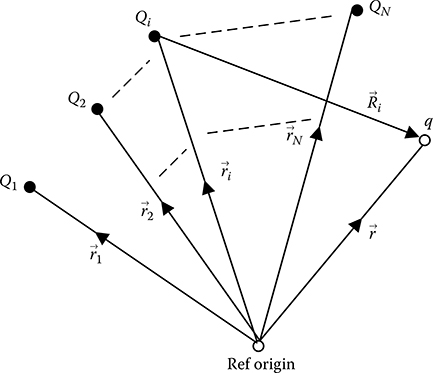
FIGURE 1.5
Force due to a system of discrete charges.

1.4.4 Force due to a System of Discrete Charges

Consider N charges, Q₁ through Q_N, which are located at position vectors ${\vec{r}}_{1}$ through ${\vec{r}}_{N}$ , as shown in Figure 1.5. Because the electrostatic forces obey the principle of superposition, the electrostatic force acting on a test charge q at position vector $\vec{r}$ is simply the vector sum of all of the forces from each of the N charges taken in isolation. Thus, the total force acting on the test charge q is given by

$\vec{F} (r) = q \sum_{i = 1}^{N} \frac{q_{i}}{4 π ε_{0}} \frac{\vec{r} - \vec{r_{i}}}{| \vec{r} - \vec{r_{i}} |^{3}} (1.6)$

where:

the distance vector ${\vec{R}}_{i} = \vec{r} - {\vec{r}}_{i}$ is directed from the ith charge Q_i to q

1.4.5 Force due to Continuous Charge Distribution

Instead of having discrete charges, consider a continuous distribution of charge represented by a charge density, which could be linear, surface or volume charge density, depending on the distribution of charge. For a continuous charge distribution, an integral over the entire region containing the charge is equivalent to a summation for infinite number of discrete charges, where each infinitesimal element of space is treated as a discrete point charge dq.

For linear charge distribution, for example, charge in a wire, considering linear charge density as λ(r′) and the infinitesimal line element dl′ at the position r′,

dq = λ(r′)dl′

For surface charge distribution, for example, charge on a plate or disc, considering surface charge density as σ(r′) and the infinitesimal area element dA′ at the position r′,

dA = σ(r′)dA′

For volume charge distribution, for example, charge in the volume of a bulk material, considering volume charge density as ρ(r′) and the infinitesimal volume element dV′ at the position r′,

dq = ρ(r′)dV′

The force on a test charge q at position r in free space is given by the integral over the entire continuous distribution of charge as follows:

$\vec{F} (r) = q \int \frac{d q}{4 π ε_{0}} \frac{\vec{r} - \bar{r'}}{| \vec{r} - \bar{r'} |^{3}} (1.7)$

In the above equation the integration is line, surface or volume integral according to the nature of charge distribution. The integral is over all space, or, at least, over all space for which the charge density is non-zero.

1.5 Electric Field Intensity

At this juncture, it is useful to define a vector field $\vec{E} (r)$ , called the electric field intensity, which is the force exerted on a unit test charge of positive polarity located at position vector $\vec{r}$ . Then, the force on a test charge could be written as follows:

$\vec{F} (r) = q \bar{E} (r) (1.8)$

The electric field intensity could be written from Equation 1.6 as follows:

$\bar{E} (r) = \sum_{i = 1}^{N} \frac{q_{i}}{4 π ε_{0}} \frac{\vec{r} - \vec{r_{i}}}{| \vec{r} - \vec{r_{i}} |^{3}} (1.9)$

or, from Equation 1.7 as follows:

$\vec{E} (r) = \int \frac{d q}{4 π ε_{0}} \frac{\vec{r} - \vec{r'}}{| \vec{r} - \vec{r'} |^{3}} (1.10)$

The electric fieldlines from a single charge Q located at a given position are purely radial and are directed outwards if the charge is positive or inwards if it is negative, as shown in Figure 1.1. Therefore, the electric field intensity at any point located at a radial distance r from the source charge Q will be the force experience by a unit test charge of positive polarity at that point and is given by

$\vec{E} (r) = \frac{Q}{4 π ε_{0} r^{2}} {\hat{u}}_{r} (1.11)$

The unit of electric field intensity as per the above definition is N/C. However, the practical unit of electric field intensity is a different one and will be discussed in Section 1.7.

1.6 Electric Flux and Electric Flux Density

Consider the case of air coming in through a window. The amount of air that comes through the window depends on the speed of the air, the direction of the air and the area of the window. The air that comes through the window may be called the air flux.

Similarly, the amount of electric fieldlines that pass through an area is the electric flux through that area. Consider the case of a source point charge of positive polarity, as shown in Figure 1.1a. If the source charge magnitude is Q C, then the total amount of electric fieldlines coming out of the source charge will be also Q C. Now, if a fictitious sphere of radius r is considered such that the source charge is located at the centre of the sphere, then the electric flux through the surface of the sphere will be Q C, as the surface of the sphere completely encloses the source charge, and all the electric fieldlines coming out radially from the source point charge passes through the spherical surface. Electric flux is typically denoted by ψ.

Electric flux density is then defined as the electric flux per unit area normal to the direction of electric flux. In the case of a point charge the electric fieldlines are directed radially from the source charge and hence the electric fieldlines are always normal to the surface of the sphere having the point charge at its center. Hence, for a point source charge of magnitude Q C, the electric flux that passes through the spherical surface area of magnitude 4π r² is Q. Then the electric flux density $(\vec{D})$ at a radial distance r from the point charge is given by

$\vec{D} (r) = \frac{Q}{4 π r^{2}} {\hat{u}}_{r} (1.12)$

From Equations 1.11 and 1.12, it may be written that

$\begin{matrix} \vec{D} (r) = ε_{0} \vec{E} (r), when the medium is free space or, \\ \vec{D} (r) = ε_{0} ε_{r} \vec{E} (r), for any particular medium of relative permittivity ε_{r} \end{matrix} (1.13)$

Electric flux density is a vector quantity because it has a direction along the electric fieldlines at the position where electric flux density is being computed.

Equation 1.13 is known as one of the basic equations of electric field theory.

However, it is not necessary that electric flux will always be normal to the area under consideration. In such cases, the component of the area that is normal to electric flux has to be taken for computing electric flux density. Figure 1.6 shows such a case, where an electric flux of magnitude ψ passes through an area of magnitude A, which is not normal to the direction of electric flux.

With reference to Figure 1.6, electric flux and electric flux density are related as follows:

$ψ = | \vec{D} | A \cos θ (1.14)$

Again, as depicted in Figure 1.6, ${\hat{u}}_{r} \cdot {\hat{u}}_{n} = \cos θ$ .

Therefore, from Equation 1.14

$ψ = | \vec{D} | A {\hat{u}}_{r} \cdot {\hat{u}}_{n} = | \vec{D} | {\hat{u}}_{r} \cdot A {\hat{u}}_{n} = \vec{D} \cdot \vec{A} (1.15)$

Images

FIGURE 1.6
Pertaining to the area related to electric flux density.

Equation 1.15 presents an important idea of introducing an area vector, which is a vector of magnitude equal to the scalar magnitude of the area under consideration, but it has a direction normal to the area under consideration. In the case of closed surfaces, area vector is conventionally taken in the direction of the outward normal. For an open surface, any one normal direction can be taken as positive, whereas the opposite normal direction is to be taken as negative.

1.7 Electric Potential

Consider that a test charge of magnitude q is located at a given position within an electric field produced by a system of charges. The test charge will experience a force due to the source charges. If the test charge moves in the direction of the field forces, then the work is done by the field forces in moving the test charge from position 1 to position 2. In other words, energy is spent by the electric field. Hence, the potential energy of test charge at position 2 will be lower than that at position 1. On the other hand, if the charge is moved against the field forces by an external agent, then the work done by the external agent will be stored as potential energy of the test charge. Hence, the potential energy of the test charge at position 2 will be higher than that at position 1. Here, it is to be noted that the force experienced by the test charge within an electric field is dependent on the magnitude of the test charge. Hence, the potential energy of the charge at any position is dependent on its magnitude and the distance by which it moves within the electric field.

The concept of electric potential is introduced to make it a property, which is purely dependent on the location within an electric field and is independent of the test charge. In other words, it is a property of the electric field itself and not related to the test particle. Hence, electric potential (ϕ) at any point within an electric field is defined as potential energy per unit charge at that point and hence it is a scalar quantity. The unit of electric potential is volt (V), which is equivalent to joules per coulomb (J/C). It is interesting to note that electric field intensity is defined as force per unit charge and electric potential is defined as potential energy per unit charge.

However, it is also practically important to note that absolute values of electric potentials are not physically measurable; only difference in potential energy between two points within an electric field can be physically measured; that is, only the potential difference between two points within an electric field is measurable. The work done in moving a unit positive charge from one point to the other within an electric field is equal to the difference in potential energies and hence difference in electric potentials at the two points.

Images

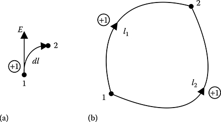
FIGURE 1.7
Pertaining to the definition of electric potential.

As shown in Figure 1.7a, consider that a unit positive charge is moved from point 1 to point 2 by a small distance dl. The force experienced by the unit positive charge at point 1 is the electric field intensity $\vec{E}$ . Then the potential difference between the ending point 2 and starting point 1 is given by

$ϕ_{2} - ϕ_{1} = - \vec{E} \cdot \vec{d l} (1.16)$

In the above equation $\vec{E} \cdot \vec{d l}$ is the work done by the field forces in moving a unit positive charge from point 1 to point 2. In this case, the potential energy of point 2 will be lower than that of point 1 and hence the potential difference (ϕ₂−ϕ₁) will be negative. For this purpose, the minus sign is introduced on the right-hand side (RHS) of Equation 1.16.

As shown in Figure 1.7b, if the unit positive charge moves through a certain distance l within an electric field from point 1 to point 2, then the magnitude as well as direction of $\vec{E}$ may not be same at every location along the path traversed by the unit positive charge. Hence, in such a case, the potential difference between point 2 and point 1 is evaluated by integrating the RHS of Equation 1.16 over the line l from point 1 to point 2 as given in Equation 1.17.

$ϕ_{2} - ϕ_{1} = - \int_{1}^{2} \vec{E} \cdot \vec{d l} (1.17)$

Equation 1.17 is known as the integral form of relationship between electric field intensity $(\vec{E})$ and electric potential (ϕ).

If point 1 is chosen at an infinite distance with respect to the source charges causing the electric field, then the potential energy at point 1 due to the source charges will be zero and hence ϕ₁ will be zero. Then Equation 1.17 can be rewritten as follows:

$ϕ_{2} = - \int_{\infty}^{2} \vec{E} \cdot \vec{d l} (1.18)$

Equation 1.18 shows that the electric potential at a point in an electric field can be defined as the work done in moving a unit positive charge from infinity to that point. Because work done is independent of the path traversed between the two end points, the electric potential is a conservative field. It is important to note here that the reference point is arbitrary and is fixed as per nature and convenience of the problem. For most of the problems, taking the reference point at infinity is a sound choice. However, for many others (e.g. a long-charged wire), a different choice may prove to be more useful. From Equation 1.18, the practical unit of electric field intensity is obtained as volt per unit length (e.g. V/m).

It is also evident from Equation 1.18 that the work done in moving a unit positive charge from infinity to a given point within an electric field could be same for several points within that electric field depending upon the distribution of electric field intensity vectors within the field region. Hence, electric potential of all such points will be same. If all these points are joined together then one may get a line or a surface on which every point has the same electric potential. Such a line or surface is called an equipotential.

Figure 1.8 shows typical examples of equipotentials in two-dimensional systems, where these will be lines. Figure 1.8a shows equipotential lines and electric fieldlines for an electric field for which $\vec{E}$ is constant everywhere, which is called uniform field. Figure 1.8b shows equipotentials and electric fieldlines for a positive polarity point charge. In this case, $\vec{E}$ varies with position and is called non-uniform field. In the case of three-dimensional systems, such equipotentials will be surfaces.

Images

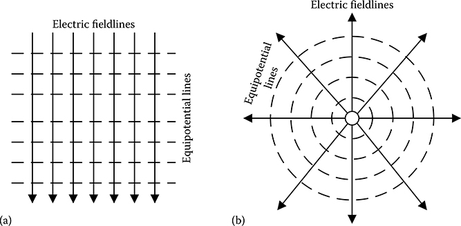
FIGURE 1.8
Examples of equipotentials: (a) uniform field and (b) non-uniform field.

Images

FIGURE 1.9
Equipotential vis-à-vis electric fieldline.

1.7.1 Equipotential vis-à-vis Electric Fieldline

Consider an equipotential of any electric field, as shown in Figure 1.9. At any point P on this equipotential, consider that the electric fieldline makes an angle θ with the tangent to the equipotential at that point. If an elementary length dl is considered along the equipotential at P, then the potential difference between the two extremities of dl will be given by $| \vec{E} | d l cos θ$ . But if dl lies on the equipotential, then there should not be any potential difference across dl. Again, the magnitude of electric field intensity is not zero at P and dl is also a non-zero quantity. Hence, the potential difference across dl could only be zero if cos θ is zero (i.e. if θ is 90°).

Thus, a basic constraint of electric field distribution is that the electric field-lines are always normal to the equipotential surface. A practical example of this constraint is that the electric fieldlines will always leave or enter conductor surfaces at 90°. This criterion is often used to check the accuracy of electric field computation by numerical techniques. The other properties of equipotential are (1) the tangential component of the electric field along the equipotential is zero and (2) no work is required to move a charged particle along an equipotential.

1.7.2 Electric Potential of the Earth Surface

The electric potential of the Earth surface could be determined with the help of the discussion in Section 1.7.1. Consider that a system of source charges has created an electric field over a region located in New York. Now, if one considers a test point on the Earth surface located in New Delhi, India, then the distance of this test point with respect to the source charges is infinite. Hence, electric potential of the test point on the Earth surface in India will be zero due to the stated source charges at New York. Now, Earth is an excellent electrical conductor and in the absence of any conductive current, the Earth surface is an equipotential. Therefore, if the test point on the Earth surface located in India is at zero potential, then all the points on the Earth surface will be at zero potential. Extending the above-mentioned logic, one may see that for any set of source charges located anywhere within this world, there will always be a point on the Earth surface that will be at infinite distance with respect to the source charges. Hence, the Earth surface potential will always be zero due to any set of source charges.

1.7.3 Electric Potential Gradient

It is defined as the positive rate of change of electric potential with respect to distance in the direction of greatest change. At any point in a field region, it will be very difficult to comprehend the direction of greatest change. To understand it conveniently, consider that the equipotentials are known within the field region. Figure 1.10 shows three such equipotentials 1, 2 and 3. Then from the point P on the equipotential 2 having an electric potential of ϕ, if one moves to any point on the equipotential having an electric potential ϕ + Δϕ, the potential difference is +Δϕ. But the minimum distance between the equipotentials 1 and 2 is the normal distance Δn. Hence, the greatest rate of change will be along the normal to the equipotential. Moreover, there are two directions of the normal to the equipotential 2 at P. Electric potential gradient is defined to be the greatest rate of change of potential in the positive sense. Hence, with reference to Figure 1.10, the electric potential gradient at P will be given by

$Electric potential gradiant (grad φ) = (Δ φ / Δ n) (1.19)$

where:

Δϕ is the potential difference
Δn is the normal distance between the two equipotentials 1 and 2 of Figure 1.10

Because electric potential gradient has magnitude along with a specific direction, it is a vector quantity and is a spatial derivative of electric potential.

1.7.4 Electric Potential Gradient and Electric Field Intensity

As discussed in Section 1.7.1, electric fieldline or $\vec{E}$ will be directed along the normal to the equipotential. But as there are two normal directions to the equipotential, the question is in which direction will $\vec{E}$ be. In this context,

Images

FIGURE 1.10
Electric potential gradient and electric field intensity.

recall that if one moves along the direction of electric field, then the potential energy decreases and hence the electric potential also decreases in the direction of electric field or $\vec{E}$ . Therefore, with reference to Figure 1.10, $\vec{E}$ will act from equipotential 2 to equipotential 3 at the point P; that is, $\vec{E}$ will act along the direction of the decreasing potential. Again, when one moves from equipotential 1 to equipotential 2 along the normal distance Δn, as shown in Figure 1.10, then the potential drop is Δϕ and the work done by the field forces is given by $| \vec{E} | Δ n$ . Hence,

$Δ ϕ = | \vec{E} | Δ n o r | \vec{E} | = \frac{Δ ϕ}{Δ n} (1.20)$

Therefore, from Equations 1.19 and 1.20, it is seen that the magnitudes of $\vec{E}$ and grad ϕ at P are the same. But, grad ϕ acts along the direction of the increasing potential and $\vec{E}$ acts along the direction of the decreasing potential and both grad ϕ and $\vec{E}$ act along the normal to the equipotential at P. Therefore, it could be concluded that

$\vec{E} = - grad ϕ (1.21)$

As shown in Figure 1.11, the potential difference (ϕ₁ – ϕ₂) between two points 1 and 2 within a field region is given by

$Δ ϕ = - \vec{E} \cdot \vec{Δ l} or Δ ϕ = - | \vec{E} | | \vec{Δ l} | cos θ (1.22)$

where:

$\vec{Δ l}$ is the distance vector from point 1 to point 2
$| \vec{E} |$ cos θ is the component of $\vec{E}$ along $\vec{Δ l}$

Images

FIGURE 1.11
Pertaining to the relationship of electric potential gradient and electric field intensity.

Now, if $\vec{Δ l}$ lies along the direction of x-axis, then Equation 1.22 can be rewritten in terms of the component of $\vec{E}$ along the x-direction, that is, E_x, and the distance Δx, as follows:

$E_{x} = - \frac{Δ ϕ}{Δ x} (1.23)$

Instead of discrete variation, for continuous variation of electric potential in x-direction, Equation 1.23 could be written in partial derivative form as follows:

$E_{x} = - \frac{\partial ϕ}{\partial x} (1.24)$

Similarly, in the y- and z-directions, E_y = −(∂ϕ/∂y) and E_z = −(∂ϕ/∂z).

Thus, the electric field intensity vector in terms of the three components could then be written as follows:

$\vec{E} = E_{x} \hat{i} + E_{y} \hat{i} + E_{z} \hat{k} = - \frac{\partial ϕ}{\partial x} \hat{i} - \frac{\partial ϕ}{\partial y} \hat{i} - \frac{\partial ϕ}{\partial z} \hat{k} = - (\frac{\partial}{\partial x} \hat{i} + \frac{\partial}{\partial y} \hat{i} + \frac{\partial}{\partial z} \hat{k}) ϕ (1.25)$

On the RHS of Equation 1.25, the vector operator within the parenthesis is the del operator, $\vec{\nabla}$ . Thus, from Equation 1.25

$\vec{E} = - \vec{\nabla} ϕ (1.26)$

The $\vec{\nabla}$ operator is an interesting operator. When it acts on a scalar quantity, the result is a vector quantity, and physically it results into the spatial derivative of the scalar quantity, that is, gradient of the scalar quantity. In this case, when $\vec{\nabla}$ acts on scalar electric potential, it results into the vector quantity electric potential gradient.

PROBLEM 1.1

The potential field in a medium having relative permittivity of 3.5 is given by ϕ = 4x³y – 5y³z + 3xz³ V. Find the electric field intensity at the point (0.1,0.5,0.2)m.

Solution:

$E_{x} = - \frac{\partial ϕ}{\partial x} = - 12 x^{2} y - 3 z^{3}$

Hence,

E_x|_{(0.1,0.5,0.2)} = −12×0.1²×0.5 − 3×0.2³ = −0.084 V/m

$E_{y} = - \frac{\partial ϕ}{\partial y} = - 4 x^{3} + 15 y^{2} z$

Hence,

E_y|_{(0.1,0.5,0.2)} = −4 × 0.1³ + 15 × 0.5² × 0.2 = 0.746 V/m

$E_{z} = - \frac{\partial ϕ}{\partial z} = 5 y^{3} - 9 x z^{2}$

Hence,

E_z|_{(0.1,0.5,0.2)} = 5 × 0.5³ − 9 × 0.1 × 0.2² = 0.589 V/m

Therefore,

$\vec{E} |_{(0.1, 0.5, 0.2)} = - 0.0 84 \hat{i} + 0.7 46 \hat{j} + 0.5 89 \hat{k} V / m$

Hence,

$| \vec{E} |_{(0.1, 0.5, 0.2)} = 0.9 54 V / m$

PROBLEM 1.2

The potential field at any point in a space containing a dielectric medium of ε_r = 5 is given by ϕ = 7x²y – 3y²z – 4z²x V, where x, y and z are in metres. Calculate the y-component of electric flux density at the point (1,4,2)m.

Solution:

$E_{y} = - \frac{\partial ϕ}{\partial y} = - 7 x^{2} + 6 y z$

Hence,

E_y|_(1,4,2) = −7 × 1² + 6 × 4 × 2 = 41 V/m

Therefore,

E_y|_(1,4,2) = 41 × 5 × 8.854 × 10⁻¹² = 1.815 nC/m²

PROBLEM 1.3

The potential field in a space containing a dielectric medium of ε_r1 is given by ϕ₁ = 7xy – 3yz – 4zx V, and another potential field in a space containing a dielectric medium of ε_r2 is given by ϕ₂ = –2x – 7yz + 5zx V, where x, y and z are in metres. If the x-component of electric flux density at the point (1,2,2)m is same in both the fields, then find the ratio of ε_r1 and ε_r2.

Solution:

$E_{x 1} = - \frac{\partial ϕ_{1}}{\partial x} = - 7 y + 4 z$

Hence,

E_x1|_(1,2,2) = −7 × 2 + 4 × 2 = −6 V/m

$E_{x 2} = - \frac{\partial ϕ_{2}}{\partial x} = 2 - 5 z$

Hence,

E_x2|_(1,2,2) = 2 − 5 × 2 = −8 V/m
Now, D_x1 = ε_r1 × ε₀ × E_x1 = −6ε_r1ε₀ C/m²
and D_x2 = ε_r2 × ε₀ × E_x2 = −8ε_r2ε₀ C/m²
As per the problem statement, D_x1 = D_x2, or, −6ε_r1ε₀ = −8ε_r2ε₀

Hence,

$\frac{ε_{r 1}}{ε_{r 2}} = 1.3 33$

1.8 Field due to Point Charge

As shown in Figure 1.12, due to a point charge +Q_i, the electric field intensity at any point P at a distance r from the charge is given by

${\vec{E}}_{r} = \frac{Q_{i}}{4 π ε_{0} r^{2}} {\hat{u}}_{r}$

If P is moved from point A to point B, as shown in Figure 1.12, then the potential difference will be as follows:

$ϕ_{B} - ϕ_{A} = - \int_{r_{A}}^{r_{B}} \frac{Q_{i}}{4 π ε_{0} r^{2}} {\hat{u}}_{r} \cdot \vec{d l} = \frac{Q_{i}}{4 π ε_{0}} (\frac{1}{r_{B}} - \frac{1}{r_{A}}) (1.27)$

If A is located at infinity, then the potential of B will be

$ϕ_{B} = \frac{Q_{i}}{4 π ε_{0} r_{B}} (1.28)$

Images

FIGURE 1.12
Field due to a point charge.

If +Q_i is located at (x_i,y_i,z_i) and B is located at (x,y,z), then

$\vec{r_{B}} = (x - x_{i}) \hat{i} + (y - y_{i}) \hat{i} + (z - z_{i}) \hat{k} (1.29)$

such that $| {\vec{r}}_{B} | = \sqrt{(x - x_{i})^{2} + (y - y_{i})^{2} + (z - z_{i})^{2}}$ and ${\hat{u}}_{r B} = \frac{{\vec{r}}_{B}}{| {\vec{r}}_{B} |}$

The electric field intensity at B will then be given by

$E_{B} = \frac{Q_{i}}{4 π ε_{0} [(x - x_{i})^{2} + (y - y_{i})^{2} + (z - z_{i})^{2}]} \frac{(x - x_{i}) \hat{i} + (y - y_{i}) \hat{i} + (z - z_{i}) \hat{k}}{[\sqrt{(x - x_{i})^{2} + (y - y_{i})^{2} + (z - z_{i})^{2}}]} (1.30)$

Hence, the three components of electric field intensity at B are (dropping the suffix B for the sake of generalization) as follows:

$\begin{array}{l} E_{x} = \frac{(x - x_{i}) Q_{i}}{4 π ε_{0} [\sqrt{(x - x_{i})^{2} + (y - y_{i})^{2} + (z - z_{i})^{2}}]^{3}} \\ E_{y} = \frac{(y - y_{i}) Q_{i}}{4 π ε_{0} [\sqrt{(x - x_{i})^{2} + (y - y_{i})^{2} + (z - z_{i})^{2}}]^{3}} \\ E_{z} = \frac{(z - z_{i}) Q_{i}}{4 π ε_{0} [\sqrt{(x - x_{i})^{2} + (y - y_{i})^{2} + (z - z_{i})^{2}}]^{3}} \end{array} (1.31)$

In the presence of multiple point charges, at any point electric potential will be the scalar sum of electric potentials and electric field intensity will be the vector sum of electric field intensities at that point due to all the charges. In other words, the effect of all the charges will be superimposed at any point within the field region.

PROBLEM 1.4

A point charge Q₁ = +1.0 μC is located at (3,1,1)m and another point charge Q₂ = –0.5 μC is located at (0.5,2,1.5)m. Find the magnitude and polarity of the point charge located at (1,2,2)m for which the z-component of electric field intensity will be zero at the origin. Medium is air.

Solution:

For the point charge 1:

Distance vector to the origin is

${\vec{r}}_{01} = (0 - 3) \hat{i} + (0 - 1) \hat{i} + (0 - 1) \hat{k} = (- 3 \hat{i} - \hat{j} - \hat{k}) m$

Therefore,

$| {\vec{r}}_{01} | = 3.317 m$

Electric field intensity at the origin:

$E_{O 1} = \frac{1 0^{- 6}}{4 π \times 1 \times ε_{0}} \times \frac{- 3 \hat{i} - \hat{j} - \hat{k}}{3. 31 7^{3}} = A (- 0.0 822 \hat{i} - 0.0 274 \hat{j} - 0.027 \hat{k}) V / m$

where:

A = 10^–6 / (4π × 1 × ε₀)

For the point charge 2:

Distance vector to the origin is

$r_{02} = (0 - 0.5) \hat{i} + (0 - 2) \hat{j} + (0 - 1.5) \hat{k} = (- 0.5 \hat{i} - 2 \hat{j} - 1.5 \hat{k}) m$

Therefore,

$| {\vec{r}}_{O 2} | = 2.5 49 m$

Electric field intensity at the origin:

$E_{O 2} = \frac{- 0.5 \times 1 0^{- 6}}{4 π \times 1 \times ε_{0}} \times \frac{- 0.5 \hat{i} - 2 \hat{j} - 1.5 \hat{k}}{2.5 4 9^{3}} = A (0.0 15 \hat{i} + 0.0 6 \hat{j} + 0.0 45 \hat{k}) V / m$

Therefore, the z-component of electric field intensity at the origin due to point charges 1 and 2 is as follows:

(−0.0274 + 0.045)A = 0.0176 AV/m

For the point charge 3, let the magnitude of the charge be Q₃ μC.

Distance vector to the origin is

${\vec{r}}_{03} = (0 - 1) \hat{i} + (0 - 2) \hat{j} + (0 - 2) \hat{k} = (- \hat{i} - 2 \hat{j} - 2 \hat{k}) m$

Therefore,

$| {\vec{r}}_{O 3} | = 3 m$

Electric field intensity at the origin:

$E_{O 3} = \frac{Q_{3} \times 1 0^{- 6}}{4 π \times 1 \times ε_{0}} \times \frac{- \hat{i} - 2 \hat{j} - 2 \hat{k}}{3^{3}} = A (- 0.0 37 \hat{i} - 0.0 74 \hat{j} - 0.074 \hat{k}) Q_{3} V / m$

If the resultant values of z-component of electric field intensity at the origin is to be zero due to the three point charges, then

−0.074AQ₃ + 0.0176A = 0, or, Q₃ = 0.238 µC

PROBLEM 1.5

Images

FIGURE 1.13
Pertaining to Problem 1.5.

A right isosceles triangle of side 1 m has charges +1, +2 and –1 nC arranged on its vertices, as shown in Figure 1.13. Find the magnitude and direction of electric field intensity at the point P, which is midway between the line connecting the +1 and –1 nC charges. Medium is air.

Solution:

Consider that a unit positive test charge is located at P.

The distance of this test charge from +1 nC is (1/√2)m.

Therefore, the electric field intensity at P due to +1 nC is $1 0^{- 9} / [4 π \times 8.8 54 \times 10^{- 12} \times (1 / \sqrt{2})^{2}] = 18 V/m$ and it acts along the line AC shown in Figure 1.13, from P to C, as it is a repulsive force on the test charge located at P.

The distance of the test charge from –1 nC is also (1/√2)m.

Therefore, the electric field intensity at P due to –1 nC is also 18 V/m and it also acts along the line AC shown in Figure 1.13 from P to C, as it is an attractive force on the test charge located at P.

The distance of this test charge from +2 nC is also (1/√2)m.

Therefore, electric field intensity at P due to +2 nC is $2 \times 1 0^{- 9} / [4 π \times 8.8 54 \times 10^{- 12} \times (1 / \sqrt{2})^{2}] = 36 V/m$ and it acts along the line BP shown in Figure 1.13 from B to P, as it is a repulsive force on the test charge located at P. BP is perpendicular to AC.

Hence, the electric field intensity acting along AC from P to C is 36 V/m and that acting along BP from B to P is also 36 V/m and these two are normal to each other.

Therefore, the resultant electric field intensity at P is $\sqrt{3 6^{2} + 3 6^{2}} = 5 0.9 1 V / m$ . It will make an angle of 45° with respect to AC. In other words, it will act along the x-axis in the positive sense of the axis.

PROBLEM 1.6

An α-particle with a kinetic energy of 1.5 MeV is projected towards a stationary platinum nucleus, which has 78 protons. Determine the distance of closest approach of the α-particle. Neglect the motion of the nucleus.

Solution:

The α-particle is positively charged. Hence, it experiences repulsive force from the nucleus and decelerates as it approaches the nucleus. At the closest approach point, it stops before being repulsed back. At this point of closest approach, all its kinetic energy is converted to potential energy.

Initial kinetic energy of the α-particle = 1.5 MeV = 1.5 × 10⁶ × 1.602 × 10^–19 J = 2.403 × 10^–13 J.

Let the distance of closest approach be d metres.

An α-particle has a charge of +3.204 × 10⁻¹⁹ C. The platinum nucleus has charge of (78 × 1.602 × 10^–19)C = +124.956 × 10^–19 C.

The electric potential at a distance of d from the platinum nucleus due to all the protons is as follows:

$\frac{78 \times 1.6 02 \times 1 0^{- 19}}{4 π \times 8.8 54 \times 1 0^{- 12} \times d} = \frac{1.1 23 \times 1 0^{- 7}}{d} V$

Hence, the potential energy of the α-particle at a distance d from platinum nucleus will be as follows:

$\frac{1.1 23 \times 1 0^{- 7}}{d} \times 3.2 04 \times 1 0^{- 19} J = \frac{3.5 98 \times 1 0^{- 26}}{d} J$

Equating this potential energy to the initial kinetic energy of 2.403 × 10^–13 J, d = 1.497 × 10^–13 m.

1.9 Field due to a Uniformly Charged Line

Figure 1.14 shows a line charge of uniform charge density λ. As a practical example, it may be considered to be a non-conducting rod, which is uniformly charged. The length of the charge is L. For the sake of simplicity, the field is computed at a point P, which is located on the line perpendicular to the line charge and passing through the midpoint of the charge. The normal distance of P from the line charge is y. For the purpose of field computation, the origin is considered to be located at the midpoint of the line charge, as shown in Figure 1.14.

Consider an elementary length of charge dx located at distance x from the origin. Then the charge on this elementary length is dq = λdx and it may be considered as a point charge.

Images

FIGURE 1.14
Field due to a uniformly charged line.

Hence, the electric potential at P due the elementary charge dq is given by

$d ϕ_{P} = \frac{d q}{4 π ε_{0} R} = \frac{λ}{4 π ε_{0}} \frac{d x}{\sqrt{(x^{2} + y^{2})}}$

Therefore, the potential at P due to the entire line charge will be as follows:

$\begin{matrix} ϕ_{P} = \frac{λ}{4 π ε_{0}} \int_{- L / 2}^{+ L / 2} \frac{d x}{\sqrt{(x^{2} + y^{2})}} = \frac{λ}{4 π ε_{0}} [\ln (x + \sqrt{x^{2} + y^{2}})]_{x = - L / 2}^{x = + L / 2} \\ or, ϕ_{P} = \frac{λ}{4 π ε_{0}} \ln \frac{\sqrt{(L / 2)^{2} + y^{2}} + (L / 2)}{\sqrt{(L / 2)^{2} + y^{2}} - (L / 2)} \end{matrix} (1.32)$

As electric potential at P is dependent only on y, hence electric field intensity at P will have only the y-component, which will be given by

$\begin{matrix} E_{y P} = - \frac{\partial ϕ_{P}}{\partial y} = \frac{λ}{4 π ε_{0}} \frac{y}{\sqrt{(L / 2)^{2} + y^{2}}} [\frac{1}{\sqrt{(L / 2)^{2} + y^{2}} - (L / 2)} - \frac{1}{\sqrt{(L / 2)^{2} + y^{2}} + (L / 2)}] \\ or, E_{y P} = \frac{λ}{4 π ε_{0}} \frac{L}{y \sqrt{(L / 2)^{2} + y^{2}}} \end{matrix} (1.33)$

The direction of electric field intensity at P along the y-axis can be explained with the help of Figure 1.14. For the elementary length of charge dx on the RHS of the origin O, another elementary length of charge can be assumed to be there at the same distance x from the origin on the left-hand side of the origin. Then the electric field intensity at P due to these two elementary charges will be same in magnitude, say dE_p. But they will be directed along the distance vectors from the elementary charges to P, as shown in Figure 1.14. They will make the same angle θ with the y-axis. Hence, the x-components of these two field intensity vectors dE_p at P will cancel each other and only the y component will be present, as the y-components of dE_p vectors will be additive at P.

1.10 Field due to a Uniformly Charged Ring

Consider a uniformly charged ring of radius a, as shown in Figure 1.15. The uniform charge density is λ. As a practical example, it may be considered to be a non-conducting annular strip of very small width, which is uniformly charged. To determine the electric potential at P located on the axis of the ring at a height of z from the plane of the ring, consider an elementary arc length adθ, as shown in Figure 1.15. Then this elementary arc length will have a charge dq = λadθ, and it may be considered as a point charge.

Images

FIGURE 1.15
Field due to a uniformly charged ring.

Hence, the electric potential at P due the elementary charge dq is given by

$d ϕ_{P} = \frac{d q}{4 π ε_{0} R} = \frac{λ}{4 π ε_{0}} \frac{a d θ}{\sqrt{(a^{2} + z^{2})}}$

Therefore, the potential at P due to the entire ring charge will be

$ϕ_{P} = \frac{λ}{4 π ε_{0}} \int_{0}^{2 π} \frac{a d θ}{\sqrt{(a^{2} + z^{2})}} (1.34)$

In the integral of Equation 1.34, it may be seen that as θ is varied from 0 to 2π along the ring, the distance R to P from any point on the ring always remains the same, that is, $\sqrt{(a^{2} + z^{2})}$ . Hence, this integral is only over θ. Therefore,

$ϕ_{P} = \frac{λ}{4 π ε_{0}} \frac{2 π a}{\sqrt{(a^{2} + z^{2})}} = \frac{λ a}{2 ε_{0} \sqrt{(a^{2} + z^{2})}} (1.35)$

Equation 1.35 shows that electric potential at P is dependent only on z; hence, electric field intensity at P will have only the z-component, which will be given by

$E_{z P} = - \frac{\partial ϕ_{P}}{\partial z} = \frac{λ}{2 ε_{0}} \frac{a z}{(a^{2} + z^{2})^{3 / 2}} (1.36)$

With the help of Figure 1.15, it can be explained why the resultant electric field intensity at the point P is directed along the z-axis. Similar to the case of a uniformly charged line, for any elementary arc length adθ, another elementary arc length adθ can be assumed to be located diametrically opposite to the first elementary arc length. Then the electric field intensity at P due to these two elementary arc lengths will be same in magnitude, say dE_p. But these two field intensity vectors of magnitude dE_p will act along the distance vectors from the two elementary arc lengths to P, as shown in Figure 1.15. It is obvious that these two vectors will make the same angle with the three axes. Hence, considering the directions of these two vectors, it can be seen that the components of electric field intensity in x- and y-directions will cancel each other, whereas the z-components will be additive in nature. Therefore, the net electric field intensity at P due to the ring charge will have only z-component.

1.11 Field due to a Uniformly Charged Disc

Consider a uniformly charged disc of radius a having a surface charge density σ, as shown in Figure 1.16. As a practical example, it may be considered to be a non-conducting disc, which is uniformly charged. Point P is located on the axis of the disc at a height z from the plane of the disc. For computing the electric potential at P, consider an annular strip of radius dr at a radius r, as shown in Figure 1.16. Then take a small arc segment of angular width dθ of this annular strip. Then this elementary surface of area dA = rdθdr will have an elementary charge dq = σdA = σrdθdr. This elementary charge dq can be considered as a point charge.

Hence, the electric potential at P due the elementary charge dq is given by

$d ϕ_{P} = \frac{d q}{4 π ε_{0} R} = \frac{σ}{4 π ε_{0}} \frac{r d θ d r}{\sqrt{(r^{2} + z^{2})}}$

Therefore, the potential at P due to the entire annular strip of charge of radius r will be

$ϕ_{P}' = \frac{σ}{4 π ε_{0}} [\int_{0}^{2 π} \frac{d θ}{\sqrt{(r^{2} + z^{2}})}] r d r (1.37)$

Images

FIGURE 1.16
Field due to a uniformly charged disc.

because, when θ varies from 0 to 2π along the annular strip of radius r, then the distance R to point P from any point on this strip remains the same, that is, $\sqrt{(r^{2} + z^{2})}$ , and the radial distance from the axis of the disc also remains the same, that is, r. Hence, the integration of Equation 1.37 is carried out over θ only. Therefore,

$ϕ_{P}' = \frac{σ}{4 π ε_{0}} \frac{2 π r d r}{\sqrt{(r^{2} + z^{2})}} = \frac{σ}{2 ε_{0}} \frac{r d r}{\sqrt{(r^{2} + z^{2})}}$

Thus, the potential at P due to the entire disc of radius a will be

$ϕ_{P} = \frac{σ}{2 ε_{0}} \int_{0}^{a} \frac{r d r}{\sqrt{(r^{2} + z^{2})}} = \frac{σ}{2 ε_{0}} [\sqrt{(r^{2} + z^{2})}]_{r = 0}^{r = a} = \frac{σ}{2 ε_{0}} [\sqrt{(a^{2} + z^{2})} - z] (1.38)$

Equation 1.38 shows that electric potential at P is dependent only on z, hence electric field intensity at P will have only the z-component, which will be given by

$E_{z P} = - \frac{\partial ϕ_{P}}{\partial z} = \frac{σ}{2 ε_{0}} [1 - \frac{z}{\sqrt{(a^{2} + z^{2})}}] (1.39)$

The charged disc comprises large number of annular strips, as shown in Figure 1.16. Each annular strip of very small radial width dr can be considered as a ring charge of uniform charge density. In Section 1.10, it has been discussed that the electric field intensity due a ring charge at any point located on the axis of the ring has only z-component. Hence, the electric field intensity at point P of Figure 1.16 due to large number of co-axial ring charges representing the annular strips of charges will also have only z-component as given by Equation 1.39.

From Equation 1.38, it may be seen that the electric potential at the centre of the disc is finite. Putting z = 0 in Equation 1.38, ϕ_O = σ a/(2ε₀).

The total charge on the entire disc is Q = πa²σ. Hence,

$ϕ_{0} = \frac{Q a}{2 π a^{2} ε_{0}} = 2 \frac{Q}{4 π ε_{0} a} (1.40)$

Equation 1.40 shows that the electric potential at the centre of the disc is equivalent to twice the work done to bring a unit positive charge from infinity to the circumference of the disc (r = a) when the entire charge of the disc is assumed to be concentrated as a point charge at the centre.

When z is very large compared to a, then

$\sqrt{z^{2} + a^{2}} = z {(1 + \frac{a^{2}}{z^{2}})}^{1 / 2} = z (1 + \frac{a^{2}}{2 z^{2}} + ...) \approx z + \frac{a^{2}}{2 z}$

Then from Equation 1.38,

$ϕ_{P} |_{z > > a} = \frac{σ}{2 ε_{0}} [z + \frac{a^{2}}{2 z} - z] = \frac{σ π a^{2}}{4 π ε_{0} z} = \frac{Q}{4 π ε_{0} z} (1.41)$

When P is located at a very large distance from the disc of finite radius a, then the disc could be considered to be a point charge of magnitude Q. Equation 1.41 is the expression for potential at a point located at distance z from a point charge of magnitude Q.

The significance of the above discussion is that the accuracy of field computation for any given charge distribution can be checked by choosing a point P, which is located sufficiently far away from the charge distribution under consideration. If the charge distribution is of finite extent, then the electric field should behave as if the charge distribution is like point charge, and decreases with the square of the distance.

PROBLEM 1.7

A circular disc of charge of radius 1 m having a uniform charge density σ = +1 nC/m² lies in the z = 0 plane, with centre at the origin. There is also a point charge of –0.4 nC at the origin. Find the magnitude and polarity of uniform charge density of a circular ring of charge of radius 1 m lying in the z = 0 plane, with centre at the origin, which would produce the same electric field intensity at the point (0,0,6)m as that due to the combined effect of the disc and point charges. Medium is air.

Solution:

As stated, the point P is located at (0,0,6)m. According to the problem statement, P lies on the axis of the disc as well as on the axis of the ring.

Hence, for the disc charge located in the x–y plane having centre at the origin:

σ = +1 nC/m², a = 1 m and z = 6 m

$E_{P - d i s c} = \frac{1 0^{- 9}}{2 \times 1 \times 8.8 54 \times 1 0^{- 12}} [1 - \frac{6}{\sqrt{(1^{2} + 6^{2})}}] = 0.7 68 V / m$

Again, for the point charge located at origin: Q = –0.4 nC, r = 6 m

$E_{P - p o i n t} = \frac{- 4 \times 1 0^{- 10}}{4 \times 1 \times 8.8 54 \times 1 0^{- 12} \times 6^{2}} = - 0.3 14 V / m$

Let the uniform charge density of the ring charge be λ C/m.

Then, for the ring charge located in x–y plane having centre at the origin, a = 1 m and z = 6 m.

$E_{P - r i n g} = \frac{λ}{2 \times 1 \times 8.8 54 \times 1 0^{- 12}} \frac{1 \times 6}{(1^{2} + 6^{2})^{3 / 2}} = 1.5 05 \times 1 0^{9} \times λ V / m$

As per the statement of the problem, E_P-ring = E_P-disc + E_P-point

or, 1.505×10⁹×λ = 0.768 − 0.314 = 0.454

Therefore, λ = 0.302 nC/m of positive polarity.

PROBLEM 1.8

Consider a ring charge of radius 10 cm and uniform charge density of λ C/m and also a disc charge of radius 15 cm and uniform charge density σ C/m². Both the two charges are placed in the x–y plane with their centre at the origin. If the electric field intensity at a point of height 20 cm lying on the z-axis is same due to the ring and disc charges individually, then find the ratio of λ and σ. Relative permittivity of the medium is 2.1.

Solution:

The point P is located at (0,0,0.2)m. Hence, it is located on the axis of both the ring and disc charges.

For the ring charge, a = 0.1 m and z = 0.2 m.

$E_{P - r i n g} = \frac{λ}{2 \times ε_{r} \times ε_{0}} \frac{0.1 \times 0.2}{(0 . 1^{2} + 0 . 2^{2})^{3 / 2}} = 0.8 94 \frac{λ}{ε_{r} ε_{0}} V / m$

For the disc charge, a = 0.15 m and z = 0.2 m.

$E_{P - d i s c} = \frac{σ}{2 \times ε_{r} \times ε_{r}} [1 - \frac{0.2}{\sqrt{(01 5^{2} + 0 2^{2})}}] = 0.1 \frac{σ}{ε_{r} ε_{r}} V / m$

But as per the problem, E_P-ring = E_P-disc

$or, 0.8 94 \frac{λ}{ε_{r} ε_{0}} = 0.1 \frac{σ}{ε_{r} ε_{0}}$

Therefore,

$\frac{λ}{σ} = 0.112$

Objective Type Questions

1. Electric field intensity is defined as

a. Force per unit charge

b. Charge per unit force

c. Potential energy per unit charge

d. Charge per unit potential energy

2. Electric potential is quantified as

a. Force per unit charge

b. Charge per unit force

c. Potential energy per unit charge

d. Charge per unit potential energy

3. Electric potential of a point may be defined as

a. Work done in moving a unit positive charge from that point to infinity

b. Work done in moving a unit positive charge from infinity to that point

c. Work done in moving a unit positive charge from the source charge to that point

d. Work done in moving a unit positive charge from that point to the source charge

4. The angle between the equipotential and electric fieldline is always

a. 0°

b. 90°

c. 180°

d. 270°

5. The conditions to be fulfilled for the validity of Coulomb’s law are:

a. The charges involved must be point charges

b. The charges should be stationary with respect to each other

c. Both (a) and (b)

d. None of the above

6. When the scalar product of two point charges is positive, then the Coulomb’s force between the charges is

a. Zero

b. Infinite

c. Repulsive

d. Attractive

7. The electrostatic force between two electric charges of magnitude 1 C separated by a distance of 1 m will be

a. ≈9 × 10⁹ N

b. ≈9 × 10^–9 N

c. ≈(1/9) × 10⁹ N

d. ≈(1/9) × 10^–9 N

8. The ratio of electrostatic to gravitational forces between two electrons separated by a given distance is approximately

a. ≈4 × 10²⁴

b. ≈(1/4) × 10²⁴

c. ≈(1/4) × 10⁴²

d. ≈4 × 10⁴²

9. If the source charge magnitude is Q coulombs, then the total amount of electric fieldlines coming out of the source charge will be

a. Q coulombs

b. (1/Q) coulombs

c. Q² coulombs

d. 1/Q² coulombs

10. For a given value of electric field intensity, if the permittivity of the medium is doubled, then the electric flux density is

a. Unchanged

b. Halved

c. Doubled

d. Squared

11. In the case of closed surfaces, area vector is conventionally taken in the direction of

a. The inward normal

b. The outward normal

c. Along the area in clockwise sense

d. Along the area in anti-clockwise sense

12. The unit of electric field intensity is

a. J/C

b. N/C

c. V/m

d. Both (b) and (c)

13. Which of the following is true as the properties of an equipotential?

a. The normal component of the electric field along the equipotential is zero

b. The tangential component of the electric field along the equipotential is zero

c. No work is required to move a particle along an equipotential

d. Both (b) and (c)

14. Which of the following quantity is zero on an equipotential?

a. Resultant electric field

b. Normal component of the electric field

c. Tangential component of the electric field

d. Electric potential

15. The angle between $\vec{E}$ and grad ϕ is

a. 0°

b. 90°

c. 180°

d. 270°

16. When $\vec{\nabla}$ acts on a scalar quantity, it results into a

a. Scalar quantity that is the spatial derivative of the scalar quantity

b. Vector quantity that is the spatial derivative of the scalar quantity

c. Scalar quantity that is the time derivative of the scalar quantity

d. Vector quantity that is the time derivative of the scalar quantity

17. In the presence of multiple point charges, electric potential and electric field intensity at any point due to all the charges will be

a. The scalar sum of electric potentials and the vector sum of electric field intensities, respectively

b. The scalar sum of electric potentials and the scalar sum of electric field intensities, respectively

c. The vector sum of electric potentials and the scalar sum of electric field intensities, respectively

d. The vector sum of electric potentials and the vector sum of electric field intensities, respectively

18. For a uniformly charged ring of positive polarity lying on the x–y plane with its axis passing through the origin, the electric field intensity at any point located on the axis is directed along

a. x-axis in the positive sense

b. y-axis in the positive sense

c. z-axis in the positive sense

d. z-axis in the negative sense

19. If the charge distribution is of finite extent, then the electric field at a point that is located sufficiently far away from the charge distribution under consideration should behave as if the charge distribution is like

a. Point charge

b. Disc charge

c. Line charge

d. Ring charge

20. The electric potential at the centre of a uniformly charged non-conducting disc is

a. Zero

b. Finite

c. Infinite

d. Undefined

21. A force $\vec{F}$ is conservative if the line integral of the force around a closed path is

a. Positive

b. Negative

c. Zero

d. Infinite

22. A uniform electric field is parallel to the z-axis. In what direction can a charge be displaced in this field without any external work being done on the charge?

a. z-axis

b. y-axis

c. x-axis

d. both (b) and (c)

23. Inside a hollow,
uniformly charged conducting sphere

a. Both electric potential and electric field intensity are zero

b. Both electric potential and electric field intensity are non-zero

c. Electric potential is zero but electric field intensity is non-zero

d. Electric potential is non-zero but electric field intensity is zero

Answers:

1) a;

2) c;

3) b;

4) b;

5) c;

6) c;

7) a;

8) d;

9) a;

10) c;

11) b;

12) d;

13) d;

14) c;

15) c;

16) b;

17) a;

18) c;

19) a;

20) b;

21) c;

22) d;

23) d

Bibliography

1. J.D. Jackson, Classical Electrodynamics, John Wiley & Sons Inc, New York, 1975.

2. M. Zahn, Electromagnetic Field Theory: A Problem Solving Approach, John Wiley & Sons Inc, New York, 1979.

3. R.K. Wangsness, Electromagnetic Fields, John Wiley & Sons Inc, New York, 1979.

4. R.S. Edgar, Field Analysis and Potential Theory, Lecture notes in engineering, Vol. 44, Springer-Verlag, USA, 1985.

5. D.K. Cheng, Field and Wave Electromagnetics, Addison-Wesley, USA, 1989.

6. P.B. Zhou, Numerical Analysis of Electromagnetic Fields, Springer-Verlag, Berlin, Heidelberg, 1993.

7. D.J. Griffiths, Introduction to Electrodynamics, Prentice Hall, New Jersey, 1999.

8. G.L. Pollack and D.R. Stump, Electromagnetism, Addison-Wesley, USA, 2002.

9. B.D. Bartolo, Classical Theory of Electromagnetism, World Scientific, New Jersey, 2004.

10. W.H. Hayt and J.A. Buck, Engineering Electromagnetics, Tata McGraw-Hill Education, New Delhi, India, 2006.

11. G.S.N. Raju, Electromagnetic Field Theory and Transmission Lines, Pearson Education, New Delhi, India, 2006.

12. U. Mukherji, Electromagnetic Field Theory and Wave Propagation, Alpha Science International, UK, 2006.

13. J. Franklin, Classical Electromagnetism, Pearson Education, New Delhi, India, 2007.

14. C.R. Paul, K.W. Whites and S.A. Nasar, Electromagnetic Fields, Tata McGraw-Hill Education, New Delhi, India, 2007.

15. G. Lehner, Electromagnetic Field Theory for Engineers and Physicists, Springer-Verlag, Berlin, Heidelberg, 2008.

16. S. Sivanagaraju and C.S. Rao, Electromagnetic Fields, New Age International, New Delhi, India, 2008.

17. K.R. Meena, Electromagnetic Fields, New Age International India, New Delhi, 2008.

18. J.R. Reitz, F.J. Milford and R.W. Christy, Foundations of Electromagnetic Theory, Pearson Education, New Delhi, India, 2009.

19. U.A. Bakshi and A.V. Bakshi, Electromagnetic Field Theory, Technical Publications, Pune, India, 2009.

20. Y. Singh, Electro Magnetic Field Theory, Pearson Education, New Delhi, India, 2011.

..................Content has been hidden....................

You can't read the all page of ebook, please click here login for view all page.

Table of Contents for 1. Fundamentals of Electric Field

Create new playlist

Sign In

Sign Up

PROBLEM 1.1

PROBLEM 1.2

PROBLEM 1.3

PROBLEM 1.4

PROBLEM 1.5

PROBLEM 1.6

PROBLEM 1.7

PROBLEM 1.8

Answers:

Table of Contents for
1. Fundamentals of Electric Field