5. Dielectric Polarization

Search in book...
Toggle Font Controls
Create new playlist

Name your new playlist

Playlist description (optional)
Sign In

Email address

Password

Forgot Password?

or

Continue with Facebook

Continue with Google
Sign Up

Full Name

Email address

Confirm Email Address

Password

or

Continue with Facebook

Continue with Google

ABSTRACT Contrary to conductors in which the charges are free to move anywhere within the material, in dielectrics, all the charges are attached to specific atoms or molecules. However, these bound charges could be displaced by a small amount under the action of an external electric field. Many dielectric materials have permanent dipoles that get aligned in the direction of the external electric field more and more as the strength of the external electric field is increased. The cumulative effect of such displacements of charges and/or alignments of dipoles determines the characteristics of dielectric materials. This chapter discusses the mechanisms by which a dielectric material gets polarized, that is, a dielectric material acquires a net dipole moment when influenced by an external electric field. The properties of dielectric materials that are intricately related to polarization are also discussed. Although a lot of dielectric materials are linear, isotropic and homogeneous (LIH), not all dielectrics exhibit such characteristics. Hence, dielectric properties of anisotropic materials are dealt elaborately in this chapter. Frequency dependence of dielectric polarization is also touched on.

5.1 Introduction

Inside any material, the electric field varies rapidly with distance in a scale corresponding to the spacing between the atoms or molecules. The local electric field at the site of an atom is significantly different from the macroscopic electric field. It is because of the fact that the local electric field acting on an atom is strongly affected by the nearest atoms, while the macroscopic field is averaged over a large number of atoms or molecules. Therefore, the determination of electric field is extremely complicated, if not impossible, at every mathematical point in a given space. As a result, the average value of electric field over a finite volume is commonly determined, particularly in the case of power engineering. This finite volume should be such that it is practically small enough to be considered as a point, but large enough to accommodate enough numbers of atoms or molecules to give smoothly varying average value of electric field.

Although conductors have large numbers of free charges that can move in response to an external electric field, the materials known as dielectrics do not have free charges inside them. Therefore, it may be argued that the dielectrics cannot have any effect of the electrostatic field. But this argument is incorrect, as the mechanism by which dielectric materials affect the electrostatic field is quite different than the mechanism in the case of conductors. Moreover, in reality, there is no electrical equipment or device without conductors as well as dielectrics. Hence, it is important from a practical viewpoint to analyze the behaviour of dielectrics in electrostatic field.

Atoms of all dielectric materials consist of charged constituents such as electrons and nucleus, which could be displaced, albeit through a small distance, by an external electric field. In the process, an electric dipole will be induced by the external electric field in a symmetrical atom or molecule, which originally had zero dipole moment. On the other hand, there are large numbers of dielectric materials containing molecules having permanent dipole moment. In those cases, the permanent dipoles will be aligned by the external electric field in its direction. The degree of alignment of permanent dipoles is higher for stronger external field. The net dipole moment of a dielectric piece is typically zero, when not influenced by external electric field, because the atoms have zero dipole moment and the permanent dipoles are randomly oriented. But due to the induction or alignment of dipoles under the action of external electric field, a dielectric piece may be considered as arrays of oriented electric dipoles. As a result, a dielectric piece acquires a net dipole moment and the dielectric is said to be polarized. The process by which a dielectric material gets polarized is known as polarization.

5.2 Field due to an Electric Dipole and Polarization Vector

A polarized dielectric can be assumed to be a collection of oriented electric dipoles situated in vacuum. If the charges of the electric dipoles and the distances between them are known, then it is possible to determine the electric potential and electric field intensity at any external location due to the polarized dielectric. But this is practically very difficult due to immensely large number of such dipoles in a polarized dielectric. Because of this reason, a kind of average dipole density is defined in the form of a vector quantity known as polarization vector for the ease of analysis.

5.2.1 Electric Dipole and Dipole Moment

When two point charges of equal magnitude but of opposite polarities are separated by a small distance, then the arrangement is known as an electric dipole, as shown in Figure 5.1. For field analysis, it is required that a single dipole be characterized by a vector quantity. As depicted in Figure 5.1, let the magnitudes of the charges be +Q and −Q, respectively, and the distance between them is d. The distance vector $\vec{d}$ between the two point charges is considered to be directed from the negative charge to the positive charge. Then the dipole moment of the electric dipole is defined as a vector

Images

FIGURE 5.1
The dipole moment of an electric dipole.

$\vec{P} = Q \vec{d} (5.1)$

The unit of dipole moment is C.m.

5.2.2 Field due to an Electric Dipole

The field due to a single electric dipole can be evaluated as the superposition of the field due to two point charges +Q and –Q, as shown in Figure 5.2. Then the electric potential at the point P due to the electric dipole is given by

$V_{P} = \frac{Q}{4 π ε_{0} r_{1}} + \frac{- Q}{4 π ε_{0} r_{2}} = \frac{Q}{4 π ε_{0}} (\frac{1}{r_{1}} - \frac{1}{r_{2}}) (5.2)$

Images

FIGURE 5.2
Field due to an electric dipole.

The distance d between the dipole charges is always much smaller than the distance of P from the two charges. Hence, the line segments r₁ and r₂ will be parallel for all practical purposes. Hence,

$r_{1} = r - \frac{d}{2} \cos θ and r_{2} = r + \frac{d}{2} \cos θ (5.3)$

where:

r = distance from the centre of the electric dipole to P
θ = the angle between the distance vectors $\vec{d}$ and $\vec{r}$

Thus, assuming r ≫ d, electric potential at a distance r from the electric dipole may be written as follows:

$V_{P} = \frac{Q d \cos θ}{4 π ε_{0} r^{2}} = \frac{\vec{p} \cdot {\hat{u}}_{r}}{4 π ε_{0} r^{2}} (5.4)$

From the above equation, it may be seen that the field due to an electric dipole is two dimensional in nature when represented in spherical coordinate system, as the field depends on r and θ coordinates and not on ϕ coordinate.

Then electric field intensity at P can be expressed as follows:

${\vec{E}}_{P} = - \vec{\nabla} V_{P} = - \frac{\partial V_{P}}{\partial r} {\hat{u}}_{r} - \frac{1}{r} \frac{\partial V_{P}}{\partial θ} {\hat{u}}_{θ} = \frac{Q d \cos θ}{2 π ε_{0} r^{3}} {\hat{u}}_{r} + \frac{Q d \sin θ}{4 π ε_{0} r^{3}} {\hat{u}}_{θ} (5.5)$

Thus, the r and θ components of electric field intensity are

$E_{r} = \frac{Q d \cos θ}{2 π ε_{0} r^{3}} and E_{θ} = \frac{Q d \sin θ}{4 π ε_{0} r^{3}} (5.6)$

Equations 5.4 and 5.5 show that electric potential and electric field intensity due to an electric dipole depend on dipole moment of the electric dipole and not on the magnitude of the charges and their separation distance separately.

5.2.3 Polarization Vector

Consider a small volume Δv of a polarized dielectric. If there are N number of molecules per unit volume in Δv and $\vec{p}$ is the average dipole moment per molecule, then as a measure of intensity of the polarization, the polarization vector, $\vec{P}$ , at a point inside Δv is defined as follows:

$\vec{P} = \frac{\sum_{Δ v} \vec{p}}{Δ v} = N \vec{p} (5.7)$

The above equation is valid for a rarefied medium, for example, a gas. The relationship needs to be written in a different way for a dense medium such as a liquid or a solid.

In a generalized manner, the net dipole moment in the small volume Δv is given by

$Q_{1} {\vec{d}}_{1} + Q_{2} {\vec{d}}_{2} + ... + Q_{N 1} {\vec{d}}_{N 1} = \sum_{i = 1}^{N 1} Q_{i} {\vec{d}}_{i} (5.8)$

where:

N1 = N × Δv

Then,

$\vec{P} = \frac{\sum_{i = 1}^{N 1} Q_{i} {\vec{d}}_{i}}{Δ v} (5.9)$

The unit of dipole moment is C.m and hence the unit of polarization vector is C/m², which is the same as that of surface charge density.

In other words, if $\vec{P}$ is known at a point, then Δv, which encloses that point and contains large number of dipoles, can be replaced by a single dipole of moment

$\vec{p} = \vec{P} Δ v (5.10)$

With the help of Equation 5.10, electric potential and electric field intensity due to a polarized dielectric can be evaluated by an integral.

5.3 Polarizability

The molecules of dielectric materials, which are the basic building blocks of the material, either have zero dipole moment or have some permanent dipole moments depending on their structure. When an external electric field is applied, then the opposite polarity charges are pulled apart and/or the permanent dipoles get aligned under the action of the external field. In this way, the dielectric material becomes polarized and this property of dielectric materials is known as polarizability.

5.3.1 Non-Polar and Polar Molecules

The molecules of a dielectric material are classified into two categories, namely, non-polar and polar. Symmetrical molecules such as CO₂, as shown in Figure 5.3c, fall in this category. In non-polar molecules the centres of gravity of positive and negative charge distribution usually coincide at one point and hence the molecules have zero dipole moment. On the other hand, a polar molecule such as H₂O and CO, as shown in Figure 5.3a and b, respectively, have permanent dipoles even in the absence of any external electric field. However, in the absence of any external field, a macroscopic piece of polar dielectric is not polarized; that is, it does not contain any dipole moment, because the molecules are randomly oriented due to thermal agitation. When the polar dielectric is subjected to an external electric field, then the individual permanent dipoles within the polar dielectric experiences torques, which tend to align these dipoles in the direction of the external field, and the dielectric gets polarized.

Images

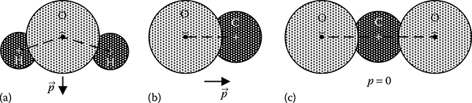
FIGURE 5.3
Non-polar and polar molecules: (a) polar H₂O; (b) polar CO and (c) non-polar CO₂.

5.3.2 Electronic Polarizability of an Atom

A simplified model of an atom is a uniformly charged electron cloud, which is spherical in shape having radius R, surrounding the total positive charge located at the point nucleus. The centres of gravity of the total negative charge (–q) of the electron cloud and the total positive charge (+q) coincides at the same point, as shown in Figure 5.4, in the absence of any external electric field.

When an external electric field is applied, the electron cloud is displaced by a small distance d until the mutual attractive force between the negatively charged electron cloud and the positively charged point nucleus balances the force due to the external electric field.

The attractive force between the electron cloud and the point nucleus is given by

$F_{i n t} = q \times \frac{(d^{3} / R^{3}) q}{4 π ε_{0} d^{2}} (5.11)$

Images

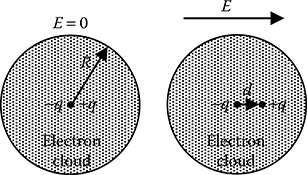
FIGURE 5.4
Electronic polarizability of an atom.

The force due to the external electric field is given by

$F_{e x t} = q E (5.12)$

At equilibrium, F_int = F_ext, or, $\frac{{dq}^{2}}{4 π ε_{0} R^{3}} = qE$

$or, d = \frac{4 π ε_{0} R^{3} E}{q} (5.13)$

Hence, the magnitude of dipole moment induced by the external electric field

$p = q d = 4 π ε_{0} R^{3} E = α_{e} E (5.14)$

where:

α_e = 4πε₀R³ = electronic polarizability of the atom

5.3.3 Types of Polarizability

The physical processes that give rise to polarizability can be subdivided into four categories: (1) electronic polarizability, (2) ionic polarizability, (3) orientational or dipolar polarizability and (4) interfacial polarizability.

5.3.3.1 Electronic Polarizability

Electronic polarizability arises due to the displacement of negatively charged electron cloud with respect to the positively charged nucleus under the influence of external electric field, as discussed in Section 5.3.2. Electronic polar-izability is present in all types of dielectric materials. It is an elastic process without any power loss and is an extremely fast process, which takes place within 10⁻¹⁶ to 10⁻¹³ s.

5.3.3.2 Ionic Polarizability

In the case of dielectric molecules that contain ionic bonds, the lengths of the bonds get stretched under the influence of the external electric field. Consider the case of NaCl, as shown in Figure 5.5. The external electric field displaces the positive Na⁺ ion towards right, whereas the negative Cl⁻ ion is displaced towards left. Thus, the forces due to external field stretch the length of the ionic bond between Na⁺ and Cl⁻ ions. As a result of the change in the length of the bond, a net dipole moment appears in the unit cell of NaCl, which does not have any dipole moment in the absence of the external electric field. Because the dipole moment in such cases arises due to the displacement of oppositely charged ions, this process is known as ionic polar-izability. Ionic polarizability exists in all dielectric materials that contain ionic bonds. Similar to electronic polarizability, ionic polarizability is also an elastic property involving no power loss. But unlike electronic polarizability, ionic polarizability is slower as ions are heavier than electrons. However, it is still a very fast process and occurs within 10⁻¹³ to 10⁻⁹ s.

Images

FIGURE 5.5
Ionic polarization in NaCl.

5.3.3.3 Orientational or Dipolar Polarizability

Although the individual molecules of a polar dielectric material have permanent dipoles, the net dipole moment becomes zero in a macroscopic piece of such dielectric material in the absence of external electric field because of random orientation of molecular dipole moments caused by thermal perturbations. Such random orientation of molecular dipoles results in near complete cancellation of dipole moment in any given direction in a macroscopic piece of polar dielectric material. But, when an external electric field is applied, then the molecular dipoles tend to align in the direction of the applied field, as shown in Figure 5.6. It is because of the fact that the energy of a dipole $\vec{p}$ placed in a local electric field ${\vec{E}}_{loc}$ is $W = - \vec{p} \cdot {\vec{E}}_{loc}$ . This energy is minimum when the dipole is oriented parallel to the applied electric field. As a result of such alignment of molecular dipoles, the net dipole moment in a macroscopic piece of polar dielectric material gets a non-zero value. This mechanism through which a non-zero dipole moment arises in a polar dielectric is known as orientational or dipolar polarizability. Dipolar polarizability is much slower than electronic or ionic polarizability, as it involves rotation of molecular dipoles that causes molecular friction. It is an inelastic process associated with power loss due to molecular friction and occurs within 10⁻⁹ to 10⁻⁴ s.

Images

FIGURE 5.6
Dipolar polarization in polar dielectric materials.

Electronic polarizability is present in all dielectrics, but the presence of ionic and dipolar polarizabilities depend on the molecular structure of dielectric materials. The relative magnitudes of the three polarizabilities, as discussed in Sections 5.3.3.1 through 5.3.3.3, are such that in non-polar, ionic dielectric materials, electronic polarizability is of the same order as ionic polarizability. On the other hand, in polar dielectric materials, the dipolar polarizability is much larger than both electronic and ionic polarizabilities.

Images

FIGURE 5.7
Interfacial polarization at dielectric interface.

5.3.3.4 Interfacial Polarizability

It occurs mainly in insulation system composed of different dielectric materials, for example, oil-impregnated paper/pressboard. Under the influence of an external electric field, small numbers of positive and negative charges, which are free to move within the bulk of the dielectric, get trapped at the interfaces of different materials, as shown in Figure 5.7, and thus produces separation of charges at the dielectric interfaces causing polarization. This mechanism known as interfacial polarizability is very slow and in general takes hours to complete.

5.4 Field due to a Polarized Dielectric

Consider a block of polarized dielectric material, as shown in Figure 5.8, containing a polarization vector $\vec{P}$ that varies with position. According to Equation 5.10, the small volume dV′ located at r′(x′, y′, z′) can be replaced by a single dipole moment $\vec{p} = \vec{P} dV'$ . Then the electric potential at any point P outside the volume of the dielectric and located at r(x,y,z) is given by

$d ϕ_{P} = \frac{\vec{P} \cdot {\hat{u}}_{R}}{4 π ε_{0} R^{2}} d V' (5.15)$

where:

$R = \sqrt{{(x - x')}^{2} + {(y - y')}^{2} + {(z - z')}^{2}}$ is the distance between the small volume dV′ and the external field point P

Images

FIGURE 5.8
Field at an external point due to a polarized dielectric.

In Equation 5.15,

$\frac{\vec{P} \cdot {\hat{u}}_{R}}{R^{2}} = \vec{P} \cdot \vec{\nabla}' (\frac{1}{R}) (5.16)$

Thus,

$d ϕ_{P} = \frac{1}{4 π ε_{0}} [\vec{P} \cdot \vec{\nabla}' (\frac{1}{R})] d V' (5.17)$

where:

$\vec{▿}'$ is the gradient with respect to the primed quantities, that is, with respect to the position of the small volume dV′ within the dielectric volume

Therefore, the potential at P due to the entire volume V of the polarized dielectric

$d ϕ_{P} = \int_{V} \frac{1}{4 π ε_{0}} [\vec{P} \cdot \vec{\nabla}' (\frac{1}{R})] d V' (5.18)$

Consider a scalar quantity a, a vector quantity $\vec{A}$ and the vector identity as follows:

$\vec{\nabla}' \cdot a \vec{A} = a \vec{\nabla}' \cdot \vec{A} + \vec{A} \cdot \vec{\nabla}' a (5.19)$

Putting a = 1/R and $\vec{A} = \vec{P}$ in the above equation, we get

$\vec{P} \cdot \vec{\nabla}' (\frac{1}{R}) = \vec{\nabla}' \cdot \frac{\vec{P}}{R} - \frac{1}{R} \vec{\nabla}' \cdot \vec{P} (5.20)$

Therefore, from Equations 5.18 and 5.20

$ϕ_{P} = \int_{V} \frac{1}{4 π ε_{0}} (\vec{\nabla}' \cdot \frac{\vec{P}}{R} - \frac{1}{R} \vec{\nabla}' \cdot \vec{P}) d V' (5.21)$

Applying the divergence theorem to the first term of the above equation,

$ϕ_{P} = \int_{S} \frac{\vec{P} \cdot {\hat{u}}_{n}^{'}}{4 π ε_{0} R} d S' + \int_{V} \frac{- \vec{\nabla}' \cdot \vec{P}}{4 π ε_{0} R} d V' (5.22)$

where:

${\hat{u}}_{n}^{'}$ is the outwards unit normal vector to the surface dS′ of the small volume dV′ of the dielectric

The two terms on the right-hand side of Equation 5.22 can be re-written as follows:

$ϕ_{P} = \frac{1}{4 π ε_{0}} [\int_{S} \frac{σ_{s b} (r')}{R} d S' + \int_{V} \frac{ρ_{v b (γ')}}{R} d V'] (5.23)$

where:

$\begin{matrix} σ_{sb} (r') = \vec{P} \cdot {\hat{u}}_{n}^{'} \\ ρ_{vb} (r') = - \vec{\nabla}' \cdot \vec{P} \end{matrix} (5.24)$

and r′ denotes the location within the polarized dielectric volume.

Then electric field intensity at P is given by

${\vec{E}}_{P} = - \vec{\nabla} ϕ_{P} = \frac{1}{4 π ε_{0}} [\int_{s} \frac{σ_{s b} (r') {\hat{u}}_{R}}{R^{2}} d S' + \int_{V} \frac{ρ_{v b} (r') {\hat{u}}_{R}}{R^{2}} d V'] (5.25)$

5.4.1 Bound Charge Densities of Polarized Dielectric

Equations 5.23 and 5.25 show that the field at an external point due to a polarized dielectric is superposition of the field due a volume charge density and a surface charge density. In other words, a polarized dielectric can be replaced by an equivalent volume charge density (ρ_vb) and an equivalent surface charge density (ρ_sb). Both volume and surface charge densities can be considered to be in vacuum, as rest of the dielectric does not produce any field at an external point. These charge densities are called bound volume charge density and bound surface charge density, respectively, as these charges appearing due to polarization are not free to move within the dielectric material. These charges are caused by displacement or rotation occurring in molecular scale during polarization. Such equivalent charge distribution is very useful because the problem of finding the field due to a polarized dielectric is converted to the problem of finding the field due to distribution of charges in vacuum, which is easier to solve. If the polarization vector is known at all the points within the polarized dielectric, then both bound volume and surface charge densities could be found from the polarization vector. Hence, the problem comes down to the determination of polarization vector within the volume of the polarized dielectric, which nowadays is done with the help of numerical techniques.

5.4.1.1 Bound Volume Charge Density

From Equation 5.24, bound volume charge density is $ρ_{vb} (r') = - \vec{▿}' \cdot \vec{P}$ , that is, if the divergence of polarization vector $\vec{P}$ is non-zero, then the bound volume charge density will exist within the volume of the polarized dielectric. For uniform polarization, divergence of $\vec{P}$ is zero and hence there could be no bound volume charge density. But for non-uniform polarization, there can be net increase or decrease of charge within a given volume. For inhomogeneous dielectrics, there will be some net volume charge, because all the molecular dipoles are not identical and hence, their effect does not cancel out on average. In such cases, the divergence of $\vec{P}$ will be non-zero and hence the bound volume charge density will be finite and non-zero. This fact can be understood from Figure 5.9a, where at the centre of the volume the negative ends of the dipoles are concentrated and hence there will be an excess of negative charges at that location giving rise to non-zero polarization vector $\vec{P}$ .

5.4.1.2 Bound Surface Charge Density

Images

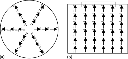
FIGURE 5.9
Equivalent charge distribution of polarized dielectric: (a) volume charge density due to nonuniform polarization, and (b) surface charge density due to uniform polarization.

From Equation 5.24, bound surface charge density is $σ_{sb} (r') = \vec{P} \cdot {\hat{u}}_{n}^{'}$ . Such surface charge densities are present for both uniform and non-uniform polarization. As shown in Figure 5.9b, in the case of uniform polarization, for a macroscopic volume of the dielectric there will be equal amount of positive and negative charges and the net charge within the volume will be zero. But if a small volume is considered that includes the upper boundary perpendicular to the direction of polarization as shown in Figure 5.9b, there will be net positive charge within the volume, no matter how thin the volume is made. In the limiting case, the thickness tends to zero, but there will still be excess positive charges on the surface. Therefore, bound charge density appears on the surface of the polarized dielectric due to uncompensated charges on the surface.

5.4.2 Macroscopic Field

The expressions for electric potential and electric field intensity due to polarized dielectric only are given by Equations 5.23 and 5.25, respectively. But the effects of the external charge distribution that causes the polarization must be added to these to get the resultant field. The effects are simply additive because the bound surface and volume charge densities due to polarization are considered to be in vacuum. Therefore, the complete expressions for electric potential and electric field intensity at a point outside the polarized dielectric due to the external charge distribution and the equivalent bound charge distributions of the polarized dielectric are given by

$ϕ_{P} = \frac{1}{4 π ε_{0}} {\int_{S} \frac{[σ_{e x t} + σ_{s b} (r')]}{R} d S' + \int_{V} \frac{[ρ_{e x t} + ρ_{v b} (r')]}{R} d V'} (5.26)$

${\vec{E}}_{P} = \frac{1}{4 π ε_{0}} {\int_{s} \frac{[σ_{e x t} + σ_{s b} (r')] {\hat{u}}_{R}}{R^{2}} d S' + \int_{V} \frac{[ρ_{e x t} + ρ_{v b} (r')] {\hat{u}}_{R}}{R^{2}} d V'} (5.27)$

5.4.3 Field due to a Narrow Column of Uniformly Polarized Dielectric

Consider a narrow column of polarized dielectric of the cross-sectional area dS with a polarization vector of magnitude P directed along the axis of the column, as shown in Figure 5.10.

Electric potential at the external point A due to the small volume dSdz of the polarized column can be expressed according to Equation 5.15 as follows:

$d ϕ_{A} = \frac{P d S d z \cos θ}{4 π ε_{0} r^{2}} = \frac{P d S d r}{4 π ε_{0} r^{2}} (5.28)$

Hence, the electric potential at A due to the entire column is

$\begin{matrix} ϕ_{A} = \frac{P d S}{4 π ε_{0}} \int_{r_{1}}^{r_{2}} \frac{d r}{r^{2}} \\ or, ϕ_{A} = \frac{P d S}{4 π ε_{0}} (\frac{1}{r_{1}} - \frac{1}{2}) = \frac{P d S}{4 π ε_{0} r_{1}} + \frac{- P d S}{4 π ε_{0} r_{2}} \end{matrix} (5.29)$

Images

FIGURE 5.10
Field due to a narrow column of uniformly polarized dielectric.

For the area dS at z₁, $\vec{P} \cdot {\hat{u}}_{n}$ is positive and that at z₂ is negative. Thus Equation 5.29 shows that the field due to the narrow column of polarized dielectric is the same as that due to positive charges (+PdS) on the surface dS at z₁ and the negative charges (−PdS) on dS at z₂. In other words, the bound charges due to polarization appear at the two surfaces as it is a case of uniform polarization.

5.4.4 Field within a Sphere Having Uniformly Polarized Dielectric

According to the discussions in Section 5.4, Equations 5.23 and 5.25 are valid if the field observation point is located outside the polarized dielectric. However, these two equations can also be applied when the field observation point is inside the polarized dielectric, provided that average electric field is determined.

Consider a sphere of radius R containing a dielectric medium of uniform polarization $\vec{P}$ . Such a uniformly polarized dielectric sphere could be equivalently constructed by superimposing two uniformly charged spheres of opposite polarity with centres displaced by a small distance d, as shown in Figure 5.11.

Electric field intensity at a radial distance r within a charged sphere of radius R is given by

$\vec{E} = \frac{q}{4 π ε_{0} r^{2}} \frac{r^{3}}{R^{3}} {\hat{u}}_{r} = \frac{q \vec{r}}{4 π ε_{0} R^{3}} (5.30)$

Images

FIGURE 5.11
Field within a uniformly polarized dielectric sphere.

where:

$\vec{r}$ points outwards from the centre of the sphere
q is the total charge within the sphere

In the case of two overlapping but slightly displaced spheres, as shown in Figure 5.11, for r < R

$\vec{E} = \frac{q {\vec{r}}_{2}}{4 π ε_{0} R^{3}} + \frac{- q \vec{r_{1}}}{4 π ε_{0} R^{3}} = \frac{q ({\vec{r}}_{2} - \vec{r_{1}})}{4 π ε_{0} R^{3}} = \frac{- q \vec{d}}{4 π ε_{0} R^{3}} (5.31)$

Considering uniform polarization, net dipole moment within the dielectric sphere is $\vec{p} = q \vec{d}$ .

Therefore, average polarization vector, $\vec{p} = (3 \vec{p}) / (4 π R^{3}) = (3 q \vec{d}) / (4 π R^{3})$ .

Therefore, from Equation 5.31,

$\vec{E} = - \frac{\vec{P}}{3 ε_{0}} (5.32)$

Electric field intensity within the sphere is the average value determined by representing the sphere as a continuum medium with uniform polarization $\vec{P}$ .

Outside the uniformly polarized sphere, electric field intensity is equivalent to that due to two point charges of opposite polarity located at the centres of the two slightly displaced spheres.

5.4.5 Sphere Having Constant Radial Distribution of Polarization

Consider a sphere of radius R with constant radial distribution of polarization, as shown in Figure 5.9a. Thus the magnitude of polarization (P) is constant but the direction changes with position within the sphere. Hence, the polarization vector within the sphere is given by $\vec{P} = P \vec{r}$ .

Polarization gives rise to bound charge density over the surface of the sphere, which is given by

$σ_{s b} = \vec{P} \cdot {\hat{u}}_{n} = P (5.33)$

Hence, total surface polarization charge is given by

$q_{s b} = 4 π R^{2} P (5.34)$

The volume charges due to polarization are distributed over the entire volume of the sphere and diverge at the centre of the sphere. The bound volume charge density can be found as follows:

$ρ_{v b} = - \vec{\nabla} \cdot \vec{P} = - P \vec{\nabla} \cdot r = - P \frac{1}{r^{2}} \frac{\partial r^{2}}{\partial r} = - \frac{2 P}{r} (5.35)$

Total volume charge due to polarization is

$q_{v b} = \int_{V} ρ_{v b} d V = \int_{0}^{R} (- \frac{2 P}{r}) 4 π r^{2} d r = - 4 π R^{2} P (5.36)$

Hence, the total polarization charge, which is the sum of the bound volume charges (q_vb) and bound surface charges (q_sb), is zero.

PROBLEM 5.1

A thin dielectric rod of cross-sectional area S extends along the z-axis from z = 0 to z = H. The polarization of the dielectric rod is along the z-axis and is given by $\vec{P} = (a_{1} z + a_{2}) \hat{k}$ . Calculate the bound surface charge density at each end, bound volume charge density and the total bound charge within the rod.

Solution:

For the surface at z = H, ${\hat{u}}_{n} = \hat{k}$ . and for the surface at z = 0, ${\hat{u}}_{n} = - \hat{k}$ .

Hence, the bound surface charge density at z = H,

$σ_{s b} |_{z = H} = \vec{P} \cdot \hat{k} |_{z = H} = (a_{1} z + a_{2}) |_{z = H} = a_{1} H + a_{2}$

and the bound surface charge density at z = 0,

$σ_{s b} |_{z = 0} = \vec{P} \cdot - \hat{k} |_{z = 0} = - (a_{1} z + a_{2}) |_{z = 0} = - a_{2}$

Therefore, total bound surface charge q_sb = (a₁H + a₂)S − a₂S = a₁HS.

The bound volume charge density $ρ_{vb} = - \vec{Δ} \cdot \vec{P} = - a_{1}$ .

Therefore, total bound volume charge q_vb = −a₁HS.

Therefore, total bound charge due to polarization = q_sb + q_vb = 0.

PROBLEM 5.2

A dielectric cube of side 2 m and centre at origin has a radial polarization given by $\vec{P} = 4 \vec{r} {nC/m}^{2}$ and $\vec{r} = 2 x \hat{i} + 2 y \hat{j} + 2 z \hat{k} m$ . Find bound surface charge density, bound volume charge density and the total bound charge due to polarization.

Solution:

Given, $\vec{P} = 8 x \hat{i} + 8 y \hat{j} + 8 z \hat{k} {nC/m.}^{2}$

For each of the six faces of the cube, there is a surface charge density σ_sb.

For the face at x = 1 m,

$σ_{s b} = \vec{P} \cdot \hat{i} |_{x = 1} = 8 x |_{x = 1} = 8 n C / m^{2}$

The magnitude of σ_sb is same for all the six faces. Therefore, considering all the six faces of the cube, total bound surface charge

q_sb 6 × 8 × 2² = 192 nC

The bound volume charge density is

$ρ_{v b} = - \vec{\nabla} \cdot \vec{P} = - (8 + 8 + 8) = - 24 n C / m^{3}$

Hence, total bound volume charge q_vb = −24 × 23 = −192 nC.

Thus, total bound charge within the cube due to polarization = 192 – 192 = 0.

5.5 Electric Displacement Vector

According to Gauss’s law,

$ε_{0} \int_{s} \vec{E} \cdot d \vec{S} = ε_{0} \int_{V} \vec{\nabla} \cdot \vec{E} d V = q_{t} (5.37)$

where:

q_t is the total charge enclosed by the volume V, which for dielectric materials include free as well as bound volume charges

Thus, $q_{t} = \int_{V} (ρ_{f} + ρ_{vb}) d V$ . Hence, from Equation 5.37

$\begin{matrix} ε_{0} \int_{V} \vec{\nabla} \cdot \vec{E} d V = \int_{V} (ρ_{f} + ρ_{v b}) d V \\ or \vec{\nabla} \cdot \vec{E} = \frac{(ρ_{f} + ρ_{v b})}{ε_{0}} = \frac{ρ_{t}}{ε_{0}} \end{matrix} (5.38)$

But, according to Equation 5.24,

$ρ_{v b} = - \vec{∇} \cdot \vec{P}$

Therefore,

$\begin{matrix} \vec{∇} \cdot \vec{E} = \frac{1}{ε_{0}} (ρ_{f} - \vec{∇} \cdot \vec{P}) \\ or, \vec{∇} \cdot (ε_{0} \vec{E} + \vec{P}) = ρ_{f} \end{matrix} (5.39)$

Equation 5.39 is very important in the sense that the divergence of the vector $(ε_{0} \vec{E} + \vec{P})$ through any volume is equal to the free charge density in that volume. This form of Gauss’s law is more convenient because the only charges that can be influenced externally are the free charges.

This vector $(ε_{0} \vec{E} + \vec{P})$ is called electric displacement vector $(\vec{D})$ , so that

$\vec{D} = ε_{0} \vec{E} + \vec{P} (5.40)$

and from Equation 5.39

$\vec{▿} \cdot \vec{D} = ρ_{f} (5.41)$

The integral form Equation 5.41 is

$\int_{s} \vec{E} \cdot d \vec{S} = \int_{V} ρ_{f} d V (5.42)$

It should be noted here that both $\vec{▿} \cdot \vec{D}$ and $\int_{s} \vec{E} \cdot d \vec{S}$ are related to free charges only and are unaffected by bound charges due to polarization.

From Equation 5.38, it may be seen that both free and bound charges are sources of $\vec{E}$ , whereas Equation 5.41 shows that only free charges are sources of $\vec{D}$ . In other words, lines of $\vec{D}$ begin and end on free charges only, but the lines of $\vec{E}$ begin and end on either free or bound charges.

From Equation 5.40, it may be written that

$\vec{E} = \frac{\vec{D}}{ε_{0}} - \frac{\vec{P}}{ε_{0}} (5.43)$

It means that the E-field within a dielectric is resultant of two fields, namely, D-field and P-field. D-field is associated with free charges, whereas P-field is associated with bound charges due to polarization. Moreover, P-field acts in opposition to D-field. Thus, in the presence of P-field, that is, in the presence of bound charges due to polarization, the E-field within a dielectric becomes less than the D-field.

5.5.1 Electric Susceptibility

For linear dielectric materials, polarization vector $\vec{P}$ varies directly with applied electric field $\vec{E}$ . Hence, $\vec{P}$ and $\vec{E}$ are related as follows:

$\vec{P} = ε_{0} χ_{e} \vec{E} (5.44)$

where:

χ_e is known as electric susceptibility of the dielectric

It is a dimensionless quantity and is a measure of how susceptible a dielectric material is to applied electric field. In other words, it indicates the relative ease of polarization of the dielectric.

5.5.2 Dielectric Permittivity

From Equations 5.40 and 5.44, for linear dielectric materials

$\vec{D} = ε_{0} (1 + χ_{e}) \vec{E} = ε_{0} ε_{r} \vec{E} (5.45)$

$o r, \vec{D} = ε \vec{E} (5.46)$

where:

$ε = ε_{0} ε_{r} (5.47)$

$ε_{r} = 1 + χ_{e} = \frac{ε}{ε_{0}} (5.48)$

where:

ε is called the permittivity
ε_r is called the dielectric constant or relative permittivity of linear dielectric and is also a dimensionless quantity

For any material in which polarization vector is non-zero, electric susceptibility is greater than unity and hence relative permittivity is always greater than unity. For the majority of dielectric materials, ε_r varies with the frequency of the applied electric field. The value of ε_r that is relevant to electrostatics is the value in steady electric field or at low frequencies (<1000 Hz).

5.5.3 Relationship between Free Charge Density and Bound Volume Charge Density

As discussed above, for linear dielectric media,

$\vec{P} = \vec{D} - ε_{0} \vec{E} = [1 - (1 / ε_{r})] \vec{D}, as \vec{D} = ε_{r} ε_{0} \vec{E}$

Therefore,

$\begin{matrix} \vec{∇} \cdot \vec{P} = (1 - \frac{1}{ε_{r}}) \vec{∇} \cdot \vec{D} = (1 - \frac{1}{ε_{r}}) ρ_{f}, as \vec{∇} \cdot \vec{D} = ρ_{f} \\ or, - ρ_{v b} = (1 - \frac{1}{ε_{r}}) ρ_{f}, as ρ_{v b} = - \vec{∇} \cdot \vec{P} \end{matrix}$

Hence, total charge density ρ_t = ρ_f + ρ_vb = (ρ_f/ε_r).

Thus for ε_r > 1, ρ_t < ρ_f, because ρ_f and ρ_vb are of opposite polarities.

PROBLEM 5.3

In a dielectric material E_y = 10 V/m and polarization vector $\vec{P} = (400 \hat{i} + 300 \hat{j} - 200 \hat{k}) p C / m^{2}$ . Calculate (1) electric susceptibility (χ_e), (2) $\vec{E}$ and (3) $\vec{D}$ .

Solution:

$\begin{matrix} P_{y} = ε_{0} χ_{e} E_{y}, or, 300 \times 1 0^{- 12} = 8.854 \times 1 0^{- 12} \times χ_{e} \times 10, or χ_{e} = 3.39 \\ E_{x} = \frac{P_{x}}{ε_{0} χ_{e}} = \frac{400 \times 1 0^{- 12}}{8.854 \times 1 0^{- 12} \times 3.39} = 13.33 V / m \\ and E_{z} = \frac{P_{z}}{ε_{0} χ_{e}} = \frac{- 200 \times 1 0^{- 12}}{8.854 \times 1 0^{- 12} \times 3.39} = - 6.67 V / m \end{matrix}$

Therefore,

$\vec{E} = (13.33 \hat{i} + 10 \hat{j} - 6.67 \hat{k}) V/m$

Now,

$\vec{D} = ε_{0} \vec{E} + \vec{P}$

Therefore,

$\begin{matrix} \vec{D} = [8.854 \times (13.33 \hat{i} + 10 \hat{j} - 6.67 \hat{k}) + (400 \hat{i} + 300 \hat{j} - 200 \hat{k})] \times 10^{- 12} {C/m}^{2} \\ or, \vec{D} = (518.02 \hat{i} + 388.54 \hat{j} - 259.05 \hat{k}) {pC/m}^{2} \end{matrix}$

5.6 Classification of Dielectrics

Equations 5.44 through 5.48 are not applicable to dielectric materials in general. These equations are valid for a sub-class of dielectric materials known as LIH materials. LIH dielectrics exhibit the following properties:

Linearity: A dielectric is said to be linear if $\vec{D}$ varies linearly with $\vec{E}$ . For such materials, permittivity is constant and independent of applied electric field. For non-linear dielectrics, $\vec{D}$ and $\vec{E}$ have non-linear relationship.
Isotropy: A dielectric is said to be isotropic if $\vec{D}$ and $\vec{E}$ are in the same direction. Isotropic dielectrics have same permittivity in all directions. For anisotropic materials, $\vec{D}, \vec{E}$ , and $\vec{P}$ are not parallel and hence permittivity varies with direction. Crystalline dielectrics are mostly anisotropic.
Homogeneity: Dielectric materials for which properties are same at all points within the volume of the material are called homogeneous. For inhomogeneous dielectrics, properties such as permittivity vary with space coordinates. A typical example of inhomogeneous dielectric is atmosphere air, as the permittivity of air varies with altitude.

5.6.1 Molecular Polarizability of Linear Dielectric

Equation 5.44 relates polarization vector $\vec{P}$ and macroscopic electric field $\vec{E}$ through electric susceptibility (χ_e) in the case of linear dielectrics. The electric field that causes polarization of a molecule of a dielectric is known as molecular field ${\vec{E}}_{mol}$ . Molecular field ${\vec{E}}_{mol}$ is different from the macroscopic field $\vec{E}$ because the polarization of neighbouring molecules gives rise to an internal field ${\vec{E}}_{int}$ .

Hence,

${\vec{E}}_{m o 1} = \vec{E} + {\vec{E}}_{i n t} (5.49)$

As shown in Figure 5.12, consider an imaginary sphere that contains the neighbouring molecules. This sphere is much larger in dimension compared to the molecules, but is infinitesimally small in macroscopic scale. The dielectric outside the sphere is replaced by the system of bound charges due to polarization (σ_sb). Then the internal field can be resolved into two components:

${\vec{E}}_{i n t} = {\vec{E}}_{n e a r} + {\vec{E}}_{f a r} (5.50)$

where:

${\vec{E}}_{n e a r}$ is the field due to neighbouring molecules, which are located close to the given molecule
${\vec{E}}_{far}$ is the field due to all other molecules, which arises from the bound charge density (σ_sb) on the sphere surface

Images

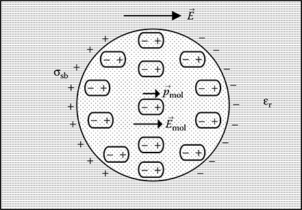
FIGURE 5.12
Molecular and macroscopic fields.

${\vec{E}}_{far}$ can be expressed in spherical coordinates as follows:

${\vec{E}}_{f a r} = \frac{1}{4 π ε_{0}} \int_{S} σ_{s b} \frac{- \vec{r}}{r^{3}} d S = \frac{1}{4 π ε_{0}} \int_{0}^{2 π} \int_{0}^{π} (P \cos θ) \frac{\vec{r}}{r^{3}} (r d θ) (r \sin θ d ϕ) (5.51)$

Considering the Cartesian coordinates, the x-component vanishes as it involves the integral $\int_{0}^{2 π} cos φ d φ$ , which evaluates to zero, and the y-component vanishes as it involves the integral $\int_{0}^{2 π} sin φ d φ$ , which is also zero. Therefore,

${\vec{E}}_{f a r} = \frac{1}{4 π ε_{0}} \int_{0}^{2 π} \int_{0}^{π} P {\hat{u}}_{z} \cos^{2} θ \sin θ d θ d ϕ = \frac{\vec{P}}{3 ε_{0}} (5.52)$

If the neighbouring molecules are randomly distributed in location, which is the case in most linear dielectrics, then ${\vec{E}}_{near} = 0$ .

Therefore,

${\vec{E}}_{i n t} = \vec{P} / (3 ε_{0})$

Then,

${\vec{E}}_{m o 1} = \vec{E} + \frac{\vec{P}}{3 ε_{0}} (5.53)$

Let N be the number of molecules per unit volume and ${\vec{p}}_{m o 1}$ be the dipole moment of each molecule, then the polarization vector $\vec{P}$ is given by

$\vec{P} = N {\vec{p}}_{m o 1} (5.54)$

Molecular dipole moment and molecular field can be related with the help of molecular polarizability (α_mol) as follows:

${\vec{p}}_{m o 1} = ε_{0} α_{m o 1} {\vec{E}}_{m o 1} (5.55)$

Hence, from Equations 5.53 through 5.55,

$\vec{P} = N ε_{0} α_{m o 1} {\vec{E}}_{m o 1} = N α_{m o 1} (ε_{0} \vec{E} + \frac{\vec{P}}{3}) (5.56)$

Putting $\vec{P} = ε_{0} χ_{e} \vec{E}$ in the above equation, we get

$χ_{e} = \frac{3 N α_{m o 1}}{3 - N α_{m o 1}} (5.57)$

Using ε_r = 1 + χ_e in the above equation, we get

$ε_{r} = 1 + \frac{3 N α_{m o 1}}{3 - N α_{m o 1}}, or α_{mol} = \frac{3}{N} \frac{(ε_{r} - 1)}{(ε_{r} + 2)} \frac{}{} (5.58)$

Equation 5.58 is known as Clausius–Mossotti relation.

In this section, we discuss a simple molecular model used to understand the linear behaviour of dielectric, that is, characteristics of a large number of dielectric materials. A detailed treatment, however, will necessitate quantum mechanical consideration.

For a non-polar dielectric, dipole moment induced by the external field is $\vec{p} = α_{e} \vec{E}$ , where, α_e = electronic polarizability of the atom. Then, polarization vector

$\vec{P} = N \vec{p}$

where:

N is the number of dipoles per unit volume

But

$\vec{P} = ε_{0} χ_{e} \vec{E}$

Hence,

$ε_{0} χ_{e} \vec{E} = N α_{e} \vec{E}, or, χ_{e} = \frac{N α_{e}}{ε_{0}}, or, ε_{r} = 1 + χ_{e} = 1 + \frac{N α_{e}}{ε_{0}} (5.59)$

5.6.2 Piezoelectric Materials

The term piezoelectricity refers to the fact that when a dielectric is mechanically stressed, then an electric field is produced within the dielectric. As a result of this electric field, measurable quantity of electric potential difference appears across the dielectric sample, which can be measured to find the mechanical strain on the dielectric. This principle is commonly used in piezoelectric strain transducers. The inverse effect also exists, that is, mechanical strain is produced in a dielectric due to the application of electric field. Piezoelectric effect is mostly reversible.

Piezoelectric materials could be natural or synthetic. The most commonly used natural piezoelectric material is quartz (SiO₂). But synthetic piezoelectric materials, for example, ceramics and polymers, are more efficient. The piezoelectric materials used in practice are berlinite (AlPO₄), gallium orthophosphate (GaPO₄), barium titanate (BaTiO₃), lead zirconate titanate (PZT: PbZr_1−xTi_xO₃), aluminium nitride (AlN) and polyvinylidene fluoride to name a few. In recent years, piezoceramics and piezopolymers are widely used in smart structures. Very recently, breakthrough in single crystal growth technique has enabled the development of high strain and high electric breakdown piezoceramics.

The nature of piezoelectric effect is strongly related to the large number of electric dipoles present in the piezoelectric materials. These dipoles can either be due to ions on crystal lattice sites with asymmetric charge distribution or due to certain molecular groups having asymmetric configurations. When a mechanical stress is applied on a piezoelectric material, the crystalline structure is disturbed and it changes the direction of the polarization vector due to the electric dipoles. If the dipole is due to the ions, then the change in polarization is caused by a re-configuration of ions within the crystalline structure. On the other hand, if the dipole is due to molecular groups, then re-orientation of molecular groups causes the change in the polarization. The electric field developed because of the change in net polarization gives rise to piezoelectric effect.

5.6.3 Ferroelectric Materials

A ferroelectric material is a dielectric with at least two discrete stable or meta-stable states of different non-zero electric polarization under zero applied electric field, referred to as spontaneous polarization. For a material to be considered ferroelectric, it must be possible to switch between these states by the application and removal of an applied electric field. In the case of conventional ferroelectrics, the spontaneous polarization is produced by the atomic arrangement of ions in the crystal structure, depending on their positions, and in electronic ferroelectrics the spontaneous polarization is produced by charge ordering of multiple valences. A non-zero spontaneous polarization can be present only in a crystal with a polar space group. Numerical values of spontaneous polarization are customarily given in units of μC/m². All ferroelectric materials are necessarily piezoelectric.

In the ferroelectric state the plot of polarization versus applied electric field shows a hysteresis loop, as shown in Figure 5.13, similar to ferromagnetic materials. A significant feature of ferroelectrics is that the spontaneous polarization can be reversed by an appropriately strong electric field applied in the opposite direction. Dielectric permittivity, which is dependent on the slope of P–E curve, is therefore dependent on the applied field, in the ferroelectric state.

Images

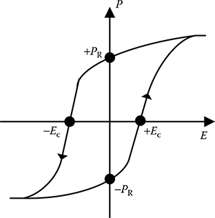
FIGURE 5.13
Hysteresis loop in ferroelectric state.

In most ferroelectrics, there is a phase transition from the ferroelectric state, to a non-polar paraelectric phase, with increasing temperature. The phase transition temperature is known as Curie point (T_C) where the ferroelectric material changes from the low temperature polarized state to high temperature unpolarized state. The spontaneous polarization in most ferroelectric crystals is greatest at temperatures well below T_C and decreases to zero at T_C. Some ferroelectric materials have no Curie point as these materials melt before the phase transition temperature is reached. The range of phase transition temperature for different ferroelectric materials is very wide varying from very low (50 ∼ 100K) to very high (over 1000K) temperature.

While ferroelectricity was discovered in hydrogen-bonded material Rochelle salt (NaKC₄H₄O₆,4H₂O), dramatic change in the understanding of this phenomenon came through the discovery of ferroelectricity in the much simpler, non-hydrogen containing, perovskite oxide BaTiO₃. BaTiO₃ is the typical example of the very large and extensively studied and used perovskite oxide family, which not only includes perovskite compounds but also includes ordered and disordered solid solutions.

Ferroelectrics are used in a variety of applications such as non-volatile memories, capacitors having tunable capacitance, varactors for radio frequency/microwave circuits, electro-optic modulators, high permittivity applications, pyroelectric detectors and so on.

5.6.4 Electrets

Electrets are unique, man-made materials that can hold an electrical charge after being polarized in an electric field. It is a piece of dielectric material that has been specially prepared to possess an overall fixed dipolarity. It is the electrical analogy of a permanent magnet. Instead of opposite magnetic poles, the electret has two electrical poles of trapped opposite polarity charges. Therefore, a fixed static potential exists between the two opposite poles of the dipolar electret.

Electrets can be prepared from different dielectric materials depending on their structures and properties. The very first electrets were made of carnauba wax (Brazilian palm gum) and its mixtures with rosin, beeswax, ethylcellulose and other components. When a polar dielectric is placed in an electric field, the applied field causes the dipoles to be oriented in such a way that the dipole moments are directed parallel to the applied field. The degree of alignment achieved depends on the freedom with which a dipole can turn around its axis. In the case of a material such as carnauba wax, this freedom is greater when the wax is in molten state, but is almost zero when the wax is in the solid state. Hence, it is possible to melt the wax, and keep it in an electric field so that the dipoles align themselves. Afterwards, while still under the influence of the electric field, the wax is allowed to cool and solidify. Then the molecular dipoles get set in the aligned position, and the wax piece becomes an electret. Electrets prepared in this way are known as thermoelectrets. It has been reported in published literature that effective surface charge density of the order of 4 ∼ 6 nC/m² has been preserved practically unchanged in carnauba wax-based electrets for more than 35 years.

However, there are several other methods of preparation of electrets: (1) photoelectrets are produced using light as heat source; (2) radioelectrets are prepared by exposing the dielectric to a beam of charged particles; (3) coronaelectret is produced by placing the dielectric in a corona discharge field and is nowadays preferred for industrial production of electrets and (4) mechanoelectrets are formed by the mechanical compression of dielectric between heated plates. Many modern electrets (such as teflon or polypropylene electrets) have only space or surface charge but no dipole polarization.

Electret materials include ceramics, non-polar/polar semi-crystalline and amorphous synthetic polymers, biopolymers and ferroelectric ceramic/polymer composites. The most common applications of electret are microphones, electro-acoustic devices, infrared detection and photocopying machines. Electrets are also being useful as novel devices in biomedical and high-energy charge storage applications.

5.7 Frequency Dependence of Polarizabilities

If the behaviour of dielectric polarizability is studied under alternating field, important distinctions between various polarizabilities emerge. Typical dependence of polarizabilities on frequency is depicted in Figure 5.14 over a wide range starting from static field to frequencies above the ultraviolet region.

Images

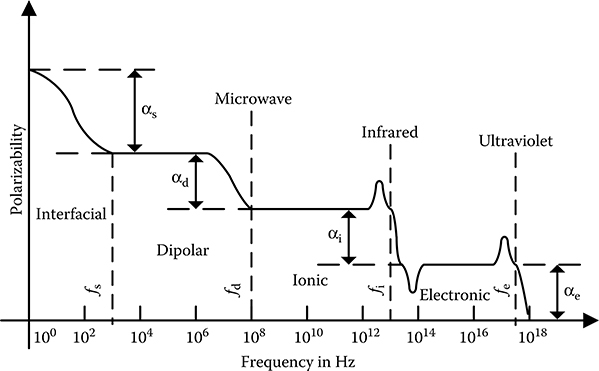
FIGURE 5.14
Frequency dependence of polarizabilities.

It may be seen that between f = 0 to f = f_s, where f_s is typically around 1 kHz, the polarizability gradually increases as frequency is decreased. Such increasing polarizability at lower frequencies arises because of interfacial polarization mechanism. From f = f_s to f = f_d, polarizability remains more or less constant, where f_d is typically in microwave region. In this frequency span, dipolar polarization mechanism is predominant. For f > f_d the polarizability decreases by a significant amount and the amount of decrease corresponds to the dipolar polar-izability. The reason for disappearance of dipolar polarizability for f > f_d is that the field at these frequencies oscillate at a rapid rate, which the dipoles are unable to follow, and hence the dipolar polarizability vanishes. Further, the polarizability remains nearly constant in the frequency range f = f_s to f = f_i, where f_i is in infrared region. The drop in polarizability for f > f_i is due to the absence of ionic polarizability at such higher frequencies, because ions being heavy are unable to follow the very rapidly varying AC field for f > f_i. As a result for f > f_i only electronic polarizability is active, because electrons being lighter are still able to follow the oscillating field at these frequencies. At extremely high frequencies for f > f_e, where f_e is in ultraviolet region, even the electronic polarizability vanishes, as the electrons are also unable to follow such extremely rapid oscillating field.

Typically, the frequencies f_e, f_i, f_d and f_s characterize electronic, ionic, dipolar and interfacial polarizabilities, respectively. These frequencies depend on the dielectric materials and vary from dielectric to dielectric and also on the condition of the dielectric. Various polarizabilities can be determined by measuring dielectric properties at various frequencies of appropriate value. In fact this principle is the foundation of frequency domain spectroscopy, which is a major technique used for condition monitoring of high-voltage insulation system.

5.8 Mass-Spring Model of Fields in Dielectrics

When an electric field is applied to a dielectric material, the nucleus is not much accelerated as it is heavy. But the electrons move in accordance with the applied field. Such a system can be modelled by the classical mass-spring model of an atom, as shown in Figure 5.15, in which the electrons are bound to nucleus like masses on springs. Let the position of the electron be denoted by x(t) and the forcing field in this direction be $\vec{E} = {\hat{u}}_{x} E_{m} e^{j ω t}$

Images

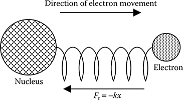
FIGURE 5.15
Mass-spring model of an atom.

Then the force acting on the electron in relation to its forced movement will be given by

$F = - c \dot{x} - k x + E_{m} e^{j ω t} (5.60)$

where:

k = spring constant
c = damping coefficient. Spring constant and damping coefficient are dependent on material

From Newton’s law of motion,

$F = m_{e} \ddot{x} (5.61)$

where:

m_e = mass of electron

From Equations 5.60 and 5.61 the equation of forced damped harmonic oscillation can be written as follows:

$m_{e} \ddot{x} + c \dot{x} + k x = q_{e} E_{m} e^{i ω t} (5.62)$

where:

q_e = charge of electron

Equation 5.62 can be rewritten as follows:

$\ddot{x} + 2 δ \dot{x} + ω_{n}^{2} x = \frac{q_{e}}{m_{e}} E_{m} e^{j ω t} (5.63)$

where:

$δ = \frac{c}{2 m_{e}} and ω_{n}^{2} = \frac{k}{m_{e}}$

To obtain the steady-state solution to Equation 5.63, let x_p(t) = x₀e^jωt. Then from Equation 5.63

$(- ω^{2} + j 2 δ ω + ω_{n}^{2}) x_{0} e^{j ω t} = \frac{q_{e}}{m_{e}} E_{m} e^{i ω t} (5.64)$

$or, χ_{0} = \frac{q_{e} E_{m}}{m_{e}} \frac{1}{(ω_{n}^{2} - ω^{2}) + i^{2 δ ω}} (5.65)$

5.8.1 Dielectric Permittivity from Mass-Spring Model

Permittivity of a linear dielectric material comprising many electrons can be derived from the mass-spring model. With respect to the rest position (x_p = 0) of the electron, the dipole moment of each electron can be written as follows:

$\vec{p} (t) = {\hat{u}}_{x} q_{e} x_{p} (t) (5.66)$

For many electrons undergoing similar motion, the polarization vector can be written as follows:

$\vec{P} (t) = N \vec{p} (t) = {\hat{u}}_{x} N q_{e} x_{p} (t) (5.67)$

where:

N is the number of dipoles per unit volume

But, according to Equation 5.44,

$\vec{P} (t) = ε_{0} χ_{e} \vec{E} (t) (5.68)$

Then from Equations 5.67 and 5.68, ${\hat{u}}_{x} N q_{e} x_{p} (t) = ε_{0} χ_{e} \vec{E} (t)$

$\begin{matrix} or, {\hat{u}}_{x} N q_{e} \frac{q_{e} E_{m}}{m_{e}} \frac{1}{(ω_{n}^{2} - ω^{2}) + i^{2 δ ω}} e^{j ω t} = {\hat{u}}_{x} ε_{0} χ_{e} E_{m} e^{j ω t} \\ or, χ_{e} = \frac{N q_{e}^{2}}{m_{e} ε_{0}} \frac{1}{(ω_{n}^{2} - ω^{2}) + i^{2 δ ω}} \end{matrix} (5.69)$

Because ε_r = 1 + χ_e, from Equation 5.69

$ε_{r} = 1 + \frac{N q_{e}^{2}}{m_{e} ε_{0}} \frac{1}{(ω_{n}^{2} - ω^{2}) + i^{2 δ ω}} (5.70)$

Although the above equation is obtained from a simple classical model, but it helps to understand several significant dielectric properties as follows:

Power loss due to the imaginary part of ε_r
Frequency dependence of permittivity
Dependence of permittivity on applied electric field
Anisotropy of dielectric materials. If the spring constants and damping coefficients are different in different directions, then permittivity will also be different in different directions.

5.9 Dielectric Anisotropy

In isotropic dielectric, D-field and E-field are in the same direction and hence $\vec{D}$ and $\vec{E}$ are related by scalar permittivity, that is, $\vec{D} = ε \vec{E}$ . But there are dielectric materials for which the stiffness of the spring, as shown in Figure 5.15, is different in different directions. It happens because of the fact that the wells of the electrostatic potential in which the charges sit are not symmetric and therefore the response of the charges is not necessarily in the direction of the forcing E-field. In other words, the charge distribution within the material responds differently to the three components of the forcing field giving rise to different permittivities in different directions.

Images

FIGURE 5.16
Polarization in anisotropic dielectric.

To explain this fact consider the material shown in Figure 5.16, which is made up of molecules that can be easily polarized by E-field acting in the y-direction but do not respond much to E-fields in the x- and z-directions. In such a material, $\vec{D}$ and $\vec{E}$ are not necessarily parallel to each other.

5.9.1 Tensor of Rank 2

If $\vec{D}$ and $\vec{E}$ are not parallel to each other, then multiplying $\vec{E}$ by a scalar will not yield $\vec{D}$ . This is because multiplying any vector by a scalar produces a new vector in the same direction having different magnitude. Multiplying any given vector by another vector with cross product will create a new vector but in a fixed direction orthogonal to both the vectors. If it is needed to change both the magnitude and direction of the given vector other than 90°, then scalar multiplication, vector products such as dot or cross products with another vector will not do. A different kind of mathematical entity has to be used for this purpose. In this case the inner product of the given vector with a dyad will be required as explained hereafter.

Consider, two vectors $A = A_{1} \hat{i} + A_{2} \hat{j} + A_{3} \hat{k}$ and $B = B_{1} \hat{i} + B_{2} \hat{j} + B_{3} \hat{k}$ . Then the dyad product of these two vectors is simply $\vec{A} \vec{B}$ . It is neither a dot nor a cross product. It may be written as

$\vec{A} \vec{B} = A_{1} B_{1} \hat{i} \hat{i} + A_{1} B_{2} \hat{i} \hat{i} + A_{1} B_{3} \hat{i} \hat{k} + A_{2} B_{1} \hat{j} \hat{i} + ... (5.71)$

where:

$\hat{i}, \hat{j}$ and $\hat{k}$ are unit vectors in the usual sense
$\hat{i} \hat{i}, \hat{i} \hat{j}, \hat{i} \hat{k}, \hat{j} \hat{i}$ and so on are unit dyads

Note that by setting A₁B₁ = α₁₁, A₁B₂ = α₁₂ and so on, the dyad $\vec{A} \vec{B}$ can be rewritten as

$\vec{A} \vec{B} = α_{11} \hat{i i} + α_{12} \hat{i} \hat{i} + α_{13} \hat{i} \hat{k} + α_{21} \hat{j} \hat{i} + ... (5.72)$

and the scalar components α_ij can be arranged in the familiar configuration of a 3 × 3 matrix:

$[\begin{matrix} α_{11} & α_{12} & α_{13} \\ α_{21} & α_{22} & α_{23} \\ α_{31} & α_{32} & α_{33} \end{matrix}] (5.73)$

Inner product of the dyad $\vec{A} \vec{B}$ and a vector $\vec{E}$ yields

$\vec{A} \vec{B} \cdot \vec{E} = \vec{A} (\vec{B} \cdot \vec{E}) = \vec{A} λ = λ \vec{A} (5.74)$

Equation 5.74 shows that the resultant vector magnitude is determined by the scalar λ and its direction is determined by $\vec{A}$ , which is not same as that of $\vec{E}$ .

In mathematical terminology, a dyad is known as tensor of rank 2. As shown by Equations 5.72 and 5.73, a tensor of rank 2 is defined as a system that has a magnitude and two directions $(\vec{A}, \vec{B})$ associated with it. It has nine components. To generalize the matter more, a scalar is a tensor of rank 0 (magnitude only and one component) and a vector is a tensor of rank 1 (magnitude, one direction and three components).

5.9.2 Permittivity Tensor

Images

FIGURE 5.17
Polarization characteristics of an anisotropic dielectric.

Consider the polarization characteristics of an anisotropic dielectric, as shown in Figure 5.17. It shows that if a forcing E-field is applied in the direction shown, then the D-field is produced in a different direction. It may be explained in the following manner. The forcing field $\vec{E}$ has three components E_x, E_y and E_z, respectively. Let the contribution to $\vec{D}$ from E_x be ${\vec{D}}_{Ex}$ . Then ${\vec{D}}_{Ex}$ can be written in terms of its three components as follows:

${\vec{D}}_{E x} = D_{x x} \hat{i} + D_{x y} \hat{j} + D_{xz} \hat{k} (5.75)$

where:

D_xx, D_xy and D_xz can be obtained by multiplying E_x with three different scalars

This is because of the fact that if an electric field E_x is applied in the x-direction, then χ_xz(=ε_xz − 1) gives the component of the additional polarization vector in the z-direction according to the relationship $\vec{P} = ε_{0} χ_{e} \vec{E}$ and similarly for the other components. Hence, Equation 5.75 can be rewritten as

${\vec{D}}_{E x} = D_{xx} \hat{i} + D_{x y} \hat{i} + D_{xz} \hat{k} = ε_{xx} E_{x} \hat{i} + ε_{x y} E_{x} \hat{i} + ε_{xz} E_{x} \hat{k} (5.76)$

Similarly, the contribution to $\vec{D}$ from E_y is ${\vec{D}}_{E y}$ , which can be written as

${\vec{D}}_{E y} = D_{y x} \hat{i} + D_{y y} \hat{i} + D_{y z} \hat{k} = ε_{y x} E_{y} \hat{i} + ε_{y y} E_{y} \hat{i} + ε_{y z} E_{y} \hat{k} (5.77)$

and the contribution to $\vec{D}$ from E_z is ${\vec{D}}_{E z}$ , which can be written as

${\vec{D}}_{E z} = D_{zx} \hat{i} + D_{z y} \hat{i} + D_{z z} \hat{k} = ε_{zx} E_{z} \hat{i} + ε_{z y} E_{z} \hat{i} + ε_{z z} E_{z} \hat{k} (5.78)$

Therefore, the net $\vec{D}$ due to $\vec{E}$ will be

$\begin{matrix} \vec{D} = & {\vec{D}}_{E x} + {\vec{D}}_{E y} + {\vec{D}}_{E z} = D_{x} \hat{i} + D_{y} \hat{j} + D_{z} \hat{k} \\ = & (D_{xx} + D_{x y} + D_{xz}) \hat{i} + (D_{y x} + D_{y y} + D_{y z}) \hat{j} + (D_{zx} + D_{z y} + D_{z z}) \hat{k} \\ = & (ε_{xx} E_{x} + ε_{x y} E_{y} + ε_{xz} E_{z}) \hat{i} + (ε_{y x} E_{x} + ε_{y y} E_{y} + ε_{y z} E_{z}) \hat{j} \\ + (ε_{zx} E_{x} + ε_{z y} E_{y} + ε_{z z} E_{z}) \hat{k} \end{matrix} (5.79)$

Equation 5.79 can be written in matrix form as follows:

$[\begin{matrix} D_{x} \\ D_{y} \\ D_{z} \end{matrix}] = [\begin{matrix} ε_{X X} & ε_{x y} & ε_{X Z} \\ ε_{y x} & ε_{y y} & ε_{y z} \\ ε_{Z X} & ε_{z y} & ε_{z z} \end{matrix}] [\begin{matrix} E_{x} \\ E_{y} \\ E_{z} \end{matrix}] (5.80)$

Referring to Equation 5.73 and introducing tensor notation, Equation 5.80 is written as

$\vec{D} = \underline{ε} \vec{E} (5.81)$

where:

$\underline{ε}$ is a tensor of rank 2 and is known as permittivity tensor of anisotropic dielectric

From Equations 5.74 and 5.81, it can be seen that the product of the tensor $\underline{ε}$ and the vector $\vec{E}$ produces a new vector $\vec{D}$ whose direction is not the same as that of E.

For an anisotropic dielectric electric susceptibility is also a tensor. Hence, Equation 5.44 is modified for an anisotropic dielectric as

$\vec{P} = ε_{0} \underline{χ_{e}} \vec{E} (5.82)$

In matrix form Equation 5.82 is written as

$[\begin{matrix} P_{x} \\ P_{y} \\ P_{z} \end{matrix}] = ε_{0} [\begin{matrix} χ_{e x x} & χ_{e x y} & χ_{e x z} \\ χ_{e y x} & χ_{e y y} & χ_{e y z} \\ χ_{e z x} & χ_{e z y} & χ_{e z z} \end{matrix}] [\begin{matrix} E_{x} \\ E_{y} \\ E_{z} \end{matrix}] (5.83)$

For a lossless dielectric, the permittivity matrix, as given in Equation 5.80, is symmetric, that is, ε_ij = ε_ji. Then Equation 5.80 can be rewritten as

$[\begin{matrix} D_{x} \\ D_{y} \\ D_{z} \end{matrix}] = [\begin{matrix} ε_{xx} & ε_{x y} & ε_{xz} \\ ε_{x y} & ε_{y y} & ε_{y z} \\ ε_{xz} & ε_{y z} & ε_{z z} \end{matrix}] [\begin{matrix} E_{x} \\ E_{y} \\ E_{z} \end{matrix}] (5.84)$

Any symmetric matrix can be diagonalized by a suitable choice for the orientation of the coordinate axes (x,y,z). The choice of coordinate axes that results in a diagonal permittivity matrix is called the principal axes of the material. In the principal axes system, Equation 5.84 can be written as

$[\begin{matrix} D_{x} \\ D_{y} \\ D_{z} \end{matrix}] = [\begin{matrix} ε_{x} & 0 & 0 \\ 0 & ε_{y} & 0 \\ 0 & 0 & ε_{z} \end{matrix}] [\begin{matrix} E_{x} \\ E_{y} \\ E_{z} \end{matrix}] (5.85)$

If the diagonal entries in Equation 5.85 are all different, that is, ε_x ≠ ε_y ≠ ε_z, then the material is called biaxial. If any two are equal, for example, ε_x ≠ ε_y = ε_z then the dielectric medium is called uniaxial.

In power engineering applications, in most of the cases LIH dielectric materials are used. For such dielectric media, all formulae derived for free space can be applied simply by replacing ε₀ with ε₀ε_r. For example, Coulomb’s law of Equation 1.1 becomes

$\vec{F} = \frac{Q_{1} Q_{2}}{4 π ε_{0} ε_{r} | \vec{r} |^{2}} {\hat{u}}_{r} (5.86)$

Objective Type Questions

1. At frequencies below 1 kHz, polarizability increases as frequency decreases. This is due to which polarization mechanism?

a. Electronic

b. Ionic

c. Dipolar

d. Interfacial

2. In the frequency range from 1 kHz to microwave region, which polarization mechanism is predominant?

a. Electronic

b. Ionic

c. Dipolar

d. Interfacial

3. Above infrared frequency range, which polarization mechanism remains active?

a. Electronic

b. Ionic

c. Dipolar

d. None of these

4. Above ultraviolet frequency range, which polarization mechanism remains active?

a. Electronic

b. Ionic

c. Dipolar

d. None of these

5. Which polarization mechanism involves power loss?

a. Electronic

b. Ionic

c. Dipolar

d. All of these

6. Which polarization occurs due to dipoles induced by applied electric field?

a. Dipolar

b. Electronic

c. Ionic

d. Both (b) and (c)

7. Which polarization takes place in the case of a non-polar dielectric?

a. Dipolar

b. Electronic

c. Ionic

d. Both (b) and (c)

8. Which polarization mechanism is slowest?

a. Interfacial

b. Dipolar

c. Ionic

d. Electronic

9. For a polar dielectric, which type of polarizability contributes maximum to the net polarizability?

a. Electronic

b. Ionic

c. Dipolar

d. None of these

10. Which type of polarization is present in any dielectric?

a. Electronic

b. Ionic

c. Dipolar

d. Interfacial

11. Electric field due to a polarized dielectric is equivalent to the field due to

a. Bound surface charge density

b. Bound volume charge density

c. Both (a) and (b)

d. None of these

12. A uniformly polarized dielectric sphere has divergent polarization directed radially outwards. Then which bound charge density will appear due to polarization?

a. Bound volume charge density

b. Bound surface charge density

c. Both (a) and (b)

d. None of these

13. Bound volume charge density due to polarization (ρ_vb) and polarization vector $(\vec{P})$ are related as

a. $ρ_{v b} = \vec{▿} \cdot \vec{P}$

b. $ρ_{v b} = - \vec{▿} \cdot \vec{P}$

c. $ρ_{v b} = | \vec{P} |$

d. $ρ_{v b} = - | \vec{P} |$

14. For a linear, isotropic dielectric, relative permittivity (ε_r) and electric susceptibility (χ_e) are related as

a. ε_r = 1 − χ_e

b. ε_r = χ_e − 1

c. ε_r = 1 + χ_e

d. ε_r = ε₀χ_e

15. For a linear, isotropic dielectric, polarization vector $(\vec{P})$ , electric susceptibility (χ_e) and applied electric field $(\vec{E})$ are related as