One of the simplest methods for clustering is to find the connected components in a graph. A connected component is a set of nodes in a graph that are connected via edges. Not all nodes need to be connected to each other to be a connected component. However, for two nodes to be in the same connected component, there needs to be a way to travel from one node to another in that connected component.

NetworkX has a function for computing connected components that we can call on our graph. First, we create a new graph using our create_graph function, but this time we pass a threshold of 0.1 to get only those edges that have a weight of at least 0.1.

G = create_graph(friends, 0.1)

We then use NetworkX to find the connected components in the graph:

sub_graphs = nx.connected_component_subgraphs(G)

To get a sense of the sizes of the graph, we can iterate over the groups and print out some basic information:

for i, sub_graph in enumerate(sub_graphs):
    n_nodes = len(sub_graph.nodes())
    print("Subgraph {0} has {1} nodes".format(i, n_nodes))

The results will tell you how big each of the connected components is. My results had one big subgraph of 62 users and lots of little ones with a dozen or fewer users.

We can alter the threshold to alter the connected components. This is because a higher threshold has fewer edges connecting nodes, and therefore will have smaller connected components and more of them. We can see this by running the preceding code with a higher threshold:

G = create_graph(friends, 0.25)
sub_graphs = nx.connected_component_subgraphs(G)
for i, sub_graph in enumerate(sub_graphs):
    n_nodes = len(sub_graph.nodes())
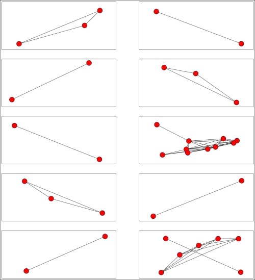
    print("Subgraph {0} has {1} nodes".format(i, n_nodes))

The preceding code gives us much smaller nodes and more of them. My largest cluster was broken into at least three parts and none of the clusters had more than 10 users. An example cluster is shown in the following figure, and the connections within this cluster are also shown. Note that, as it is a connected component, there were no edges from nodes in this component to other nodes in the graph (at least, with the threshold set at 0.25):

We can graph the entire set too, showing each connected component in a different color. As these connected components are not connected to each other, it actually makes little sense to plot these on a single graph. This is because the positioning of the nodes and components is arbitrary, and it can confuse the visualization. Instead, we can plot each separately on a separate subfigure.

In a new cell, obtain the connected components and also the count of the connected components:

sub_graphs = nx.connected_component_subgraphs(G)
n_subgraphs = nx.number_connected_components(G)

Create a new pyplot figure and give enough room to show all of our connected components. For this reason, we allow the graph to increase in size with the number of connected components:

fig = plt.figure(figsize=(20, (n_subgraphs * 3)))

Next, iterate over each connected component and add a subplot for each. The parameters to add_subplot are the number of rows of subplots, the number of columns, and the index of the subplot we are interested in. My visualization uses three columns, but you can try other values instead of three (just remember to change both values):

for i, sub_graph in enumerate(sub_graphs):
    ax = fig.add_subplot(int(n_subgraphs / 3), 3, i)

By default, pyplot shows plots with axis labels, which are meaningless in this context. For that reason, we turn labels off:

    ax.get_xaxis().set_visible(False)
    ax.get_yaxis().set_visible(False)

Then we plot the nodes and edges (using the ax parameter to plot to the correct subplot). To do this, we also need to set up a layout first:

    pos = nx.spring_layout(G)
    nx.draw_networkx_nodes(G, pos, sub_graph.nodes(), ax=ax, node_size=500)
    nx.draw_networkx_edges(G, pos, sub_graph.edges(), ax=ax)

The results visualize each connected component, giving us a sense of the number of nodes in each and also how connected they are.

Our algorithm for finding these connected components relies on the threshold parameter, which dictates whether edges are added to the graph or not. In turn, this directly dictates how many connected components we discover and how big they are. From here, we probably want to settle on some notion of which is the best threshold to use. This is a very subjective problem, and there is no definitive answer. This is a major problem with any cluster analysis task.

We can, however, determine what we think a good solution should look like and define a metric based on that idea. As a general rule, we usually want a solution where:

The Silhouette Coefficient is a metric that quantifies these points. Given a single sample, we define the Silhouette Coefficient as follows:

Where a is the intra-cluster distance or the average distance to the other samples in the sample's cluster, and b is the inter-cluster distance or the average distance to the other samples in the next-nearest cluster.

To compute the overall Silhouette Coefficient, we take the mean of the Silhouettes for each sample. A clustering that provides a Silhouette Coefficient close to the maximum of 1 has clusters that have samples all similar to each other, and these clusters are very spread apart. Values near 0 indicate that the clusters all overlap and there is little distinction between clusters. Values close to the minimum of -1 indicate that samples are probably in the wrong cluster, that is, they would be better off in other clusters.

Using this metric, we want to find a solution (that is, a value for the threshold) that maximizes the Silhouette Coefficient by altering the threshold parameter. To do that, we create a function that takes the threshold as a parameter and computes the Silhouette Coefficient.

We then pass this into the optimize module of SciPy, which contains the minimize function that is used to find the minimum value of a function by altering one of the parameters. While we are interested in maximizing the Silhouette Coefficient, SciPy doesn't have a maximize function. Instead, we minimize the inverse of the Silhouette (which is basically the same thing).

The scikit-learn library has a function for computing the Silhouette Coefficient, sklearn.metrics.silhouette_score; however, it doesn't fix the function format that is required by the SciPy minimize function. The minimize function requires the variable parameter to be first (in our case, the threshold value), and any arguments to be after it. In our case, we need to pass the friends dictionary as an argument in order to compute the graph. The code is as follows:

def compute_silhouette(threshold, friends):

We then create the graph using the threshold parameter, and check it has at least some nodes:

    G = create_graph(friends, threshold=threshold)
    if len(G.nodes()) < 2:

The Silhouette Coefficient is not defined unless there are at least two nodes (in order for distance to be computed at all). In this case, we define the problem scope as invalid. There are a few ways to handle this, but the easiest is to return a very poor score. In our case, the minimum value that the Silhouette Coefficient can take is -1, and we will return -99 to indicate an invalid problem. Any valid solution will score higher than this. The code is as follows:

        return -99 

We then extract the connected components:

    sub_graphs = nx.connected_component_subgraphs(G)

The Silhouette is also only defined if we have at least two connected components (in order to compute the inter-cluster distance), and at least one of these connected components has two members (to compute the intra-cluster distance). We test for these conditions and return our invalid problem score if it doesn't fit. The code is as follows:

    if not (2 <= nx.number_connected_components() < len(G.nodes()) - 1):
        return -99

Next, we need to get the labels that indicate which connected component each sample was placed in. We iterate over all the connected components, noting in a dictionary which user belonged to which connected component. The code is as follows:

label_dict = {}
for i, sub_graph in enumerate(sub_graphs):
    for node in sub_graph.nodes():
        label_dict[node] = i

Then we iterate over the nodes in the graph to get the label for each node in order. We need to do this two-step process, as nodes are not clearly ordered within a graph but they do maintain their order as long as no changes are made to the graph. What this means is that, until we change the graph, we can call .nodes() on the graph to get the same ordering. The code is as follows:

labels = np.array([label_dict[node] for node in G.nodes()])

Next the Silhouette Coefficient function takes a distance matrix, not a graph. Addressing this is another two-step process. First, NetworkX provides a handy function to_scipy_sparse_matrix, which returns the graph in a matrix format that we can use:

X = nx.to_scipy_sparse_matrix(G).todense()

The Silhouette Coefficient implementation in scikit-learn, at the time of writing, doesn't support sparse matrices. For this reason, we need to call the todense() function. Typically, this is a bad idea—sparse matrices are usually used because the data typically shouldn't be in a dense format. In this case, it will be fine because our dataset is relatively small; however, don't try this for larger datasets.

However, the values are based on our weights, which are a similarity and not a distance. For a distance, higher values indicate more difference. We can convert from similarity to distance by subtracting the value from the maximum possible value, which for our weights was 1:

    X = 1 - X

Now we have our distance matrix and labels, so we have all the information we need to compute the Silhouette Coefficient. We pass the metric as precomputed; otherwise, the matrix X will be considered a feature matrix, not a distance matrix (feature matrices are used by default nearly everywhere in scikit-learn). The code is as follows:

    return silhouette_score(X, labels, metric='precomputed')

We have one small problem, though. This function returns the Silhouette Coefficient, which is a score where higher values are considered better. Scipy's optimize module only defines a minimize function, which works off a loss function where lower scores are better. We can fix this by inverting the value, which takes our score function and returns a loss function.

def inverted_silhouette(threshold, friends):
    return -compute_silhouette(threshold, friends)

This function creates a new function from an original function. When the new function is called, all of the same arguments and keywords are passed onto the original function and the return value is returned, except that this returned value is negated before it is returned.

Now we can do our actual optimization. We call the minimize function on the inverted compute_silhouette function we defined:

result = minimize(inverted_silhouette, 0.1, args=(friends,))

The parameters are as follows:

Running this function, I got a threshold of 0.135 that returns 10 components. The score returned by the minimize function was -0.192. However, we must remember that we negated this value. This means our score was actually 0.192. The value is positive, which indicates that the clusters tend to be more separated than not (a good thing). We could run other models and check whether it results in a better score, which means that the clusters are better separated.

We could use this result to recommend users—if a user is in a connected component, then we can recommend other users in that component. This recommendation follows our use of the Jaccard Similarity to find good connections between users, our use of connected components to split them up into clusters, and our use of the optimization technique to find the best model in this setting.

However, a large number of users may not be connected at all, so we will use a different algorithm to find clusters for them.