
9.2 Macroeconometric Factor Models
For macroeconomic factor models, the factors are observed and we can apply the least-squares method to the MLR model in Eq. (9.4) to perform estimation. The estimate is
![]()
from which the estimates of ![]() and
and ![]() are readily available. The residuals of Eq. (9.4) are
are readily available. The residuals of Eq. (9.4) are
![]()
Based on the model assumption, the covariance matrix of ![]() is estimated by
is estimated by
![]()
where ![]() is the (i, i)th element of
is the (i, i)th element of ![]() . Furthermore, the R2 of the ith asset of Eq. (9.3) is
. Furthermore, the R2 of the ith asset of Eq. (9.3) is
![]()
where ![]() denotes the (i, i)th element of the matrix
denotes the (i, i)th element of the matrix ![]() .
.
Note that the aforementioned least-squares estimation does not impose the constraint that the specific factors ![]() are uncorrelated with each other. Consequently, the estimates obtained are not efficient in general. However, imposing the orthogonalization constraint requires nontrivial computation and is often ignored. One can check the off-diagonal elements of the matrix
are uncorrelated with each other. Consequently, the estimates obtained are not efficient in general. However, imposing the orthogonalization constraint requires nontrivial computation and is often ignored. One can check the off-diagonal elements of the matrix ![]() to verify the adequacy of the fitted model. These elements should be close to zero.
to verify the adequacy of the fitted model. These elements should be close to zero.
9.2.1 Single-Factor Model
The best known macroeconomic factor model in finance is the market model; see Sharpe (1970). This is a single-factor model and can be written as
9.5 ![]()
where rit is the excess return of the ith asset, rmt is the excess return of the market, and βi is the well-known β for stock returns. To illustrate, we consider monthly returns of 13 stocks and use the return of the S&P 500 index as the market return. The stocks used and their tick symbols are given in Table 9.1, and the sample period is from January 1990 to December 2003 so that k = 13 and T = 168. We use the monthly series of 3-month Treasury bill rates of the secondary market as the risk-free interest rate to obtain simple excess returns of the stock and market index. The returns are in percentages.
Table 9.1 Stocks Used and Their Tick Symbols in Analysis of Single-Factor Modela

aSample means (standard errors) of excess returns are also given. The sample period is from January 1990 to December 2003.
We use S-Plus to implement the estimation method discussed in the previous section. Most of the commands used also apply to the software R.
> x=read.matrix(“m-fac9003.txt”,header=T)
> xmtx=cbind(rep(1,168),x[,14])
> rtn=x[,1:13]
> xit.hat=solve(xmtx,rtn)
> beta.hat=t(xit.hat[2,])
> E.hat=rtn-xmtx%*%xit.hat
> D.hat=diag(crossprod(E.hat)/(168-2))
> r.square=1-(168-2)*D.hat/diag(var(rtn,SumSquares=T))
The estimates of βi, ![]() , and R2 for the ith asset return are given below:
, and R2 for the ith asset return are given below:
> t(rbind(beta.hat,sqrt(D.hat),r.square))
beta.hat sigma(i) r.square
AA 1.292 7.694 0.347
AGE 1.514 7.808 0.415
CAT 0.941 7.725 0.219
F 1.219 8.241 0.292
FDX 0.805 8.854 0.135
GM 1.046 8.130 0.238
HPQ 1.628 9.469 0.358
KMB 0.550 6.070 0.134
MEL 1.123 6.120 0.388
NYT 0.771 6.590 0.205
PG 0.469 6.459 0.090
TRB 0.718 7.215 0.157
TXN 1.796 11.474 0.316
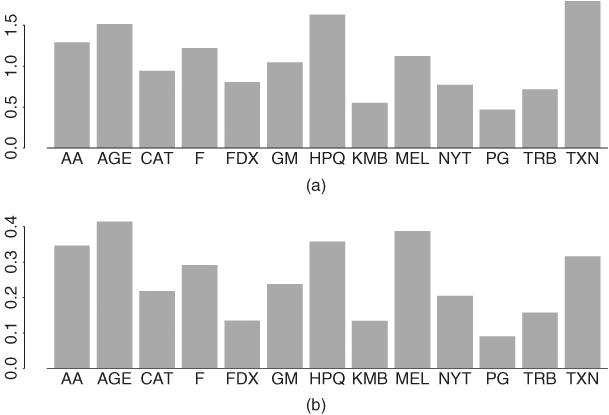
Figure 9.1 shows the bar plots of ![]() and R2 of the 13 stocks. The financial stocks, AGE and MEL, and the high-tech stocks, HPQ and TXN, seem to have higher β and R2. On the other hand, KMB and PG have lower β and R2. The R2 ranges from 0.09 to 0.41, indicating that the market return explains less than 50% of the variabilities of the individual stocks used.
and R2 of the 13 stocks. The financial stocks, AGE and MEL, and the high-tech stocks, HPQ and TXN, seem to have higher β and R2. On the other hand, KMB and PG have lower β and R2. The R2 ranges from 0.09 to 0.41, indicating that the market return explains less than 50% of the variabilities of the individual stocks used.
Figure 9.1 Bar plots of (a) beta and (b) R2 for fitting single-factor market model to monthly excess returns of 13 stocks. S&P 500 index excess return is used as market index. Sample period is from January 1990 to December 2003.
The covariance and correlation matrices of ![]() under the market model can be estimated using the following:
under the market model can be estimated using the following:
> cov.r=var(x[,14])*(t(beta.hat)%*%beta.hat)+diag(D.hat)
> sd.r=sqrt(diag(cov.r))
> corr.r=cov.r/outer(sd.r,sd.r)
> print(corr.r,digits=1,width=2)
AA AGE CAT F FDX GM HPQ KMB MEL NYT PG TRB TXN
AA 1.0 0.4 0.3 0.3 0.2 0.3 0.4 0.2 0.4 0.3 0.2 0.2 0.3
AGE 0.4 1.0 0.3 0.3 0.2 0.3 0.4 0.2 0.4 0.3 0.2 0.3 0.4
CAT 0.3 0.3 1.0 0.3 0.2 0.2 0.3 0.2 0.3 0.2 0.1 0.2 0.3
F 0.3 0.3 0.3 1.0 0.2 0.3 0.3 0.2 0.3 0.2 0.2 0.2 0.3
FDX 0.2 0.2 0.2 0.2 1.0 0.2 0.2 0.1 0.2 0.2 0.1 0.1 0.2
GM 0.3 0.3 0.2 0.3 0.2 1.0 0.3 0.2 0.3 0.2 0.1 0.2 0.3
HPQ 0.4 0.4 0.3 0.3 0.2 0.3 1.0 0.2 0.4 0.3 0.2 0.2 0.3
KMB 0.2 0.2 0.2 0.2 0.1 0.2 0.2 1.0 0.2 0.2 0.1 0.1 0.2
MEL 0.4 0.4 0.3 0.3 0.2 0.3 0.4 0.2 1.0 0.3 0.2 0.2 0.3
NYT 0.3 0.3 0.2 0.2 0.2 0.2 0.3 0.2 0.3 1.0 0.1 0.2 0.3
PG 0.2 0.2 0.1 0.2 0.1 0.1 0.2 0.1 0.2 0.1 1.0 0.1 0.2
TRB 0.2 0.3 0.2 0.2 0.1 0.2 0.2 0.1 0.2 0.2 0.1 1.0 0.2
TXN 0.3 0.4 0.3 0.3 0.2 0.3 0.3 0.2 0.3 0.3 0.2 0.2 1.0
We can compare these estimated correlations with the sample correlations of the excess returns.
> print(cor(rtn),digits=1,width=2)
AA AGE CAT F FDX GM HPQ KMB MEL NYT PG TRB TXN
AA 1.0 0.3 0.6 0.5 0.2 0.4 0.5 0.3 0.4 0.4 0.1 0.3 0.5
AGE 0.3 1.0 0.3 0.3 0.3 0.3 0.3 0.3 0.4 0.4 0.2 0.2 0.3
CAT 0.6 0.3 1.0 0.4 0.2 0.3 0.2 0.3 0.4 0.3 0.1 0.4 0.3
F 0.5 0.3 0.4 1.0 0.3 0.6 0.3 0.3 0.4 0.4 0.1 0.3 0.3
FDX 0.2 0.3 0.2 0.3 1.0 0.2 0.3 0.3 0.2 0.2 0.1 0.3 0.2
GM 0.4 0.3 0.3 0.6 0.2 1.0 0.3 0.3 0.4 0.2 0.1 0.3 0.3
HPQ 0.5 0.3 0.2 0.3 0.3 0.3 1.0 0.1 0.3 0.3 0.1 0.2 0.6
KMB 0.3 0.3 0.3 0.2 0.3 0.3 0.1 1.0 0.3 0.2 0.3 0.3 0.1
MEL 0.4 0.4 0.4 0.4 0.2 0.4 0.3 0.4 1.0 0.3 0.4 0.3 0.3
NYT 0.4 0.4 0.3 0.4 0.3 0.2 0.3 0.2 0.3 1.0 0.2 0.5 0.2
PG 0.1 0.2 0.1 0.1 0.1 0.1 0.1 0.3 0.4 0.2 1.0 0.3 0.1
TRB 0.3 0.2 0.4 0.3 0.3 0.3 0.2 0.3 0.3 0.5 0.3 1.0 0.2
TXN 0.5 0.3 0.3 0.3 0.2 0.3 0.6 0.1 0.3 0.2 0.1 0.2 1.0
In finance, one can use the concept of global minimum variance portfolio (GMVP) to compare the covariance matrix implied by a fitted factor model with the sample covariance matrix of the returns. For a given covariance matrix ![]() , the global minimum variance portfolio is the portfolio
, the global minimum variance portfolio is the portfolio ![]() that solves
that solves
![]()
where ![]() is the variance of the portfolio. The solution is given by
is the variance of the portfolio. The solution is given by
![]()
where ![]() is the k-dimensional vector of ones.
is the k-dimensional vector of ones.
For the market model considered, the GMVP for the fitted model and the data are as follows:
> w.gmin.model=solve(cov.r)%*%rep(1,nrow(cov.r))
> w.gmin.model=w.gmin.model/sum(w.gmin.model)
> t(w.gmin.model)
AA AGE CAT F FDX GM
[1,] 0.0117 -0.0306 0.0792 0.0225 0.0802 0.0533
HPQ KMB MEL NYT PG TRB TXN
[1,] -0.0354 0.2503 0.0703 0.1539 0.2434 0.1400 -0.0388
> w.gmin.data=solve(var(rtn))%*%rep(1,nrow(cov.r))
> w.gmin.data=w.gmin.data/sum(w.gmin.data)
> t(w.gmin.data)
AA AGE CAT F FDX GM
[1,] -0.0073 -0.0085 0.0866 -0.0232 0.0943 0.0916
HPQ KMB MEL NYT PG TRB TXN
[1,] 0.0345 0.2296 0.0495 0.1790 0.2651 0.0168 -0.0080
Comparing the two GMVPs, the weights assigned to TRB stock differ markedly. The two portfolios, however, have larger weights for KMB, NYT, and PG stocks.
Finally, we examine the residual covariance and correlation matrices to verify the assumption that the special factors are not correlated among the 13 stocks. The first four columns of the residual correlation matrix are given below and there exist some large values in the residual cross correlations, for example, Cor(CAT,AA) = 0.45 and Cor(GM,F) = 0.48.
> resi.cov=t(E.hat)%*%E.hat/(168-2)
> resi.sd=sqrt(diag(resi.cov))
> resi.cor=resi.cov/outer(resi.sd,resi.sd)
> print(resi.cor,digits=1,width=2)
AA AGE CAT F
AA 1.00 -0.13 0.45 0.22
AGE -0.13 1.00 -0.03 -0.01
CAT 0.45 -0.03 1.00 0.23
F 0.22 -0.01 0.23 1.00
FDX 0.00 0.14 0.05 0.07
GM 0.14 -0.09 0.15 0.48
HPQ 0.24 -0.13 -0.07 -0.00
KMB 0.16 0.06 0.18 0.05
MEL -0.02 0.06 0.09 0.10
NYT 0.13 0.10 0.07 0.19
PG -0.15 -0.02 -0.01 -0.07
TRB 0.12 -0.02 0.25 0.16
TXN 0.19 -0.17 0.09 -0.02
9.2.2 Multifactor Models
Chen, Roll, and Ross (1986) consider a multifactor model for stock returns. The factors used consist of unexpected changes or surprises of macroeconomic variables. Here unexpected changes denote the residuals of the macroeconomic variables after removing their dynamic dependence. A simple way to obtain unexpected changes is to fit a VAR model of Chapter 8 to the macroeconomic variables. For illustration, we consider the following two monthly macroeconomic variables:
1. Consumer price index (CPI) for all urban consumers: all items and with index 1982−1984 = 100.
2. Civilian employment numbers 16 years and over (CE16): measured in thousands.
Both CPI and CE16 series are seasonally adjusted, and the data span is from January 1975 to December 2003. We use a longer period to obtain the surprise series of the variables. For both series, we construct the growth rate series by taking the first difference of the logged data. The growth rates are in percentages.
To obtain the surprise series, we use the BIC criterion to identify a VAR(3) model. Thus, the two macroeconomic factors used in the factor model are the residuals of a VAR(3) model from 1990 to 2003. For the excess returns, we use the same 13 stocks as before. Details of the analysis follow:
> da=read.table('m-cpice16-dp7503.txt’),header=T)
> cpi=da[,1]
> cen=da[,2]
> x1=cbind(cpi,cen)
> y1=data.frame(x1)
> ord.choice=VAR(y1,max.ar=13)
> ord.choice$info
ar(1) ar(2) ar(3) ar(4) ar(5) ar(6)
BIC 36.992 38.093 28.234 46.241 60.677 75.810
ar(7) ar(8) ar(9) ar(10) ar(11) ar(12) ar(13)
BIC 86.23 99.294 111.27 125.46 138.01 146.71 166.92
> var3.fit=VAR(x1˜ar(3))
> res=var3.fit$residuals[166:333,1:2]
> da=matrix(scan(file='m-fac9003.txt’),14)
> xmtx = cbind(rep(1,168),res)
> da=t(da)
> rtn=da[,1:13]
> xit.hat=solve(xmtx,rtn)
> beta.hat=t(xit.hat[2:3,])
> E.hat=rtn - xmtx%*%xit.hat
> D.hat=diag(crossprod(E.hat)/(168-3))
> r.square=1-(168-3)*D.hat/diag(var(rtn,SumSquares=T))
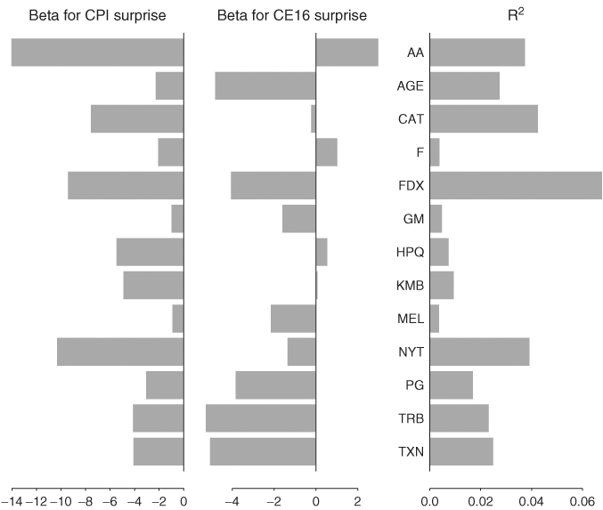
Figure 9.2 shows the bar plots of the beta estimates and R2 for the 13 stocks. It is interesting to see that all excess returns are negatively related to the unexpected changes of CPI growth rate. This seems reasonable. However, the R2 of all excess returns are low, indicating that the two macroeconomic variables used have very little explanatory power in understanding the excess returns of the 13 stocks.
Figure 9.2 Bar plots of betas and R2 for fitting two-factor model to monthly excess returns of 13 stocks. Sample period is from January 1990 to December 2003.
The estimated covariance and correlation matrices of the two-factor model can be obtained using the following:
> cov.rtn=beta.hat%*%var(res)%*%t(beta.hat)+diag(D.hat)
> sd.rtn=sqrt(diag(cov.rtn))
> cor.rtn = cov.rtn/outer(sd.rtn,sd.rtn)
> print(cor.rtn,diits=1,width=2)
The correlation matrix is very close to the identity matrix, indicating that the two-factor model used does not fit the excess returns well. Finally, the correlation matrix of the residuals of the two-factor model is given by the following:
> cov.resi=t(E.hat)%*%E.hat/(168-3)
> sd.resi=sqrt(diag(cov.resi))
> cor.resi=cov.resi/outer(sd.resi,sd.resi)
> print(cor.resi,digits=1,width=2)
As expected, this correlation matrix is close to that of the original excess returns given before and is omitted.