11.3 Model Transformation

To appreciate the flexibility of the state-space model, we rewrite some well-known econometric and financial models in state-space form.

11.3.1 CAPM with Time-Varying Coefficients

First, consider the capital asset pricing model (CAPM) with time-varying intercept and slope. The model is

11.29

where rt is the excess return of an asset, rM, t is the excess return of the market, and the innovations {et, ηt, ϵt} are mutually independent. This CAPM allows for time-varying α and β that evolve as a random walk over time. We can easily rewrite the model as

Thus, the time-varying CAPM is a special case of the state-space model with st = Tt = Rt, = It the 2 × 2 identity matrix, dt = 0, ct = 0, Zt, = (1,r,m,t), and . Furthermore, in the form of Eq. (11.28), we have εt = 0, ut = ηt,εt,et

If diffuse initialization is used, then

SsfPack/S-Plus Specification of Time-Varying Models

For the CAPM in Eq. (11.29), Φt contains rM, t, which is time varying. Some special input is required to specify such a model in SsfPack. Basically, it requires two additional variables: (a) a data matrix X that stores Zt and (b) an index matrix for Φt that identifies Zt from the data matrix. The notation for index matrices of the state-space model in Eq. (11.28) is given in Table 11.3. Note that the matrix JΦ must have the same dimension as ΦA. The elements of JΦ are all set to − 1 except the elements for which the corresponding elements of Φt are time varying. The nonnegative index value of JΦ indicates the column of the data matrix X, which contains the time-varying values.

Table 11.3 Notation and Name Used in SsfPack/S-Plus for Time-Varying State-Space Model

Index Matrix	Name Used in SsfPack/S-Plus
Jδ	mJDelta
JΦ	mJPhi
JΩ	mJOmega
Time-Varying Data Matrix	Name Used in SsfPack/S-Plus
X	mX

To illustrate, consider the monthly simple excess returns of General Motors stock from January 1990 to December 2003 used in Chapter 9. The monthly simple

excess return of the S&P 500 composite index is used as the market return. The specification of a time-varying CAPM requires values of the variances , , and . Suppose that (ση, σϵ, σe) = (0.02, 0.04, 0.1). The state-space specification for the CAPM under SsfPack/S-Plus is given below:

11.3.2 ARMA Models

Consider a zero-mean ARMA(p, q) process yt of Chapter 2:

11.30

where and , and p and q are nonnegative integers. There are many ways to transform such an ARMA model into a state-space form. We discuss three methods available in the literature. Let m = max(p, q + 1) and rewrite the ARMA model in Eq. (11.30) as

11.31

where ϕi = 0 for i > p and θj = 0 for j > q. In particular, θm = 0 because m > q.

Akaike's Approach

Akaike (1975) defines the state vector st as the minimum collection of variables that contains all the information needed to produce forecasts at the forecast origin t. It turns out that, for the ARMA process in Eq. (11.30) with m = max(p, q + 1) st = (ytIt, yt+tI1, …, yt+m-1It)′, where yt+j|t = E(yt+j|Ft) is the conditional expectation of yt+j given Ft = {y1, … , yt}. Since yt|t = yt, the first element of st is yt. Thus, the observation equation is

11.32

where . We derive the transition equation in several steps. First, from the definition,

11.33

where sit is the ith element of . Next, consider the MA representation of ARMA models given in Chapter 2. That is,

where ψ0 = 1 and other ψ weights can be obtained by equating coefficients of Bi in . In particular, we have

11.34

Using the MA representation, we have, for j > 0,

and

Thus, for j > 0, we have

11.35

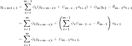
This result is referred to as the forecast updating formula of ARMA models. It provides a simple way to update the forecast from origin t to origin t + 1 when yt+1 becomes available. The new information of yt+1 is contained in the innovation at+1, and the time-t forecast is revised based on this new information with weight ψj−1 to compute the time-(t + 1) forecast.

Finally, from Eq. (11.31) and using E(at+j|Ft+1) = 0 for j > 1, we have

Taking Eq. (11.35), the prior equation becomes

11.36

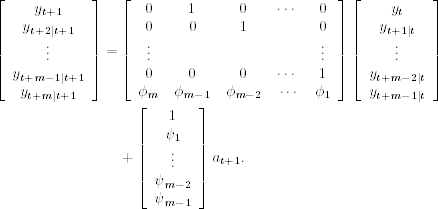
where the last equality uses Eq. (11.34). Combining Eqs. (11.33) and (11.35) for j = 2, … , m − 1, and (11.36) together, we have

11.37

Thus, the transition equation of Akaike's approach is

11.38

where ηt = at+1, and T and R are the coefficient matrices in Eq. (11.37).

Harvey's Approach

Harvey (1993, Section 4.4) provides a state-space form with an m-dimensional state vector st, the first element of which is yt, that is, s1t = yt. The other elements of st are obtained recursively. From the ARMA(m, m − 1) model, we have

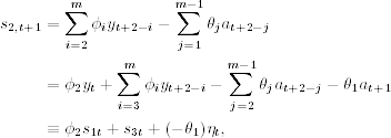
where , ηt = at+1, and as defined earlier s1t = yt. Focusing on s2, t+1, we have

where . Next, considering s3, t+1, we have

where . Repeating the procedure, we have . Finally,

Putting the prior equations together, we have a state-space form

11.39

11.40

where the system matrices are time invariant defined as Z = (1, 0,…,0 )1xm,

and dt, ct, and Ht are all zero. The model in Eqs. (11.39) and (11.40) has no measurement errors. It has an advantage that the AR and MA coefficients are directly used in the system matrices.

Aoki's Approach

Aoki (1987, Chapter 4) discusses several ways to convert an ARMA model into a state-space form. First, consider the MA model, that is, yt = θ(B)at. In this case, we can simply define st = (at-q,at-q+2,…, at-1)′, and obtain the state-space form

11.41

Note that, in this particular case, at appears in both state and measurement equations.

Next, consider the AR model, that is, ϕ(B)zt = at. Aoki (1987) introduces two methods. The first method is a straightfoward one by defining st = (zt−p+1, … , zt)′ to obtain

11.42

The second method defines the state vector in the same way as the first method except that at is removed from the last element; that is, st = zt - at if p = 1 and st = (zt-p+1,…, zt-1,zt- at)′ if p > 1. Simple algebra shows that

11.43

Again, at appears in both transition and measurement equations.

Turn to the ARMA(p, q) model ϕ(B)yt = θ(B)at. For simplicity, we assume q < p and introduce an auxiliary variable zt = [1/ϕ(B)]at. Then, we have

Since zt is an AR(p) model, we can use the transition equation in Eq. (11.42) or (11.43). If Eq. (11.42) is used, we can use yt = θ(B)zt to construct the measurement equation as

11.44

where it is understood that p > q and θj = 0 for j > q. On the other hand, if Eq. (11.43) is used as the transition equation, we construct the measurement equation as

11.45

In summary, there are many state-space representations for an ARMA model. Each representation has its pros and cons. For estimation and forecasting purposes, one can choose any one of those representations. On the other hand, for a time-invariant coefficient state-space model in Eqs. (11.26) and (11.27), one can use the Cayley–Hamilton theorem to show that the observation yt follows an ARMA(m, m) model, where m is the dimension of the state vector.

SsfPack Command

In SsfPack/S-Plus, a command GetSsfArma can be used to transform an ARMA model into a state-space form. Harvey's approach is used. To illustrate, consider the AR(1) model

The state-space form of the model is

Since the AR(1) model is stationary, the program uses ∑1I0 = Var(yt) = (0.4)2/ (1 − 0.62) = 0.25 and μ1I0 = 0. These values appear in the matrix mSigma.

As a second example, consider the ARMA(2,1) model

The state-space form of the model is

As expected, the output shows that

and mPhi and mOmega follow the format of Eq. (11.28), and the covariance matrix of (s1t, s2t)′ is used in mSigma, where s1t = yt and s2t = − 0.35yt−1 − 0.25yt−2. Note that in SsfPack, the MA polynomial of an ARMA model assumes the form θ(B) = 1 + θ1B + … + θqBq, not the form θ(B) = 1 − θ1B − … − θqBq commonly used in the literature.

11.3.3 Linear Regression Model

Multiple linear regression models can also be represented in state-space form. Consider the model

where xt is a p-dimensional explanatory variable and β is a p-dimensional parameter vector. Let βt for all t. Then the model can be written as

11.46

Thus, the system matrices are Tt = Ip, Zt, = xt′, ct = 0, Qt = 0, and . Since the state vector is fixed, a diffuse initialization should be used.

One can extend the regression model so that βt is random, say,

and Rt = (σ1, …,σp)′ with σi ≥ 0. If σi = 0, then βi is time invariant.

SsfPack Command

In SsfPack, the command GetSsfReg creates a state-space form for the multiple linear regression model. The command has an input argument that contains the data matrix of explanatory variables. To illustrate, consider the simple market model

where rt is the return of an asset and rM, t is the market return, for example, the S&P 500 composite index return. The state-space form can be obtained as

11.3.4 Linear Regression Models with ARMA Errors

Consider the regression model with ARMA(p, q) errors:

11.47

where and is a k-dimensional vector of explanatory variables. A special case of this model is the nonzero mean ARMA(p, q) model in which xt = 1 for all t and becomes a scalar parameter. Let be a state vector for the zt series, for example, that defined in Eq. (11.39). We can define a state vector for yt as

11.48

where βt = β for all t. Then, a state-space form for yt is

11.49

11.50

where , m = max(p, q + 1), and

where T and R are defined in Eq. (11.39). In a compact form, we have the state-space model

SsfPack Command

SsdPack uses the command GetSsfRegArma to construct a state-space form for linear regression models with ARMA errors. The arguments of the command can be found using the command args(GetSsfRegArma). They consist of a data matrix for the explanatory variables and ARMA model specification. To illustrate, consider the model

We use the notation X to denote the T × 2 matrix of regressors (1, xt). A state-space form for the prior model can be obtained as

11.3.5 Scalar Unobserved Component Model

The basic univariate unobserved component model, or the structural time series model (STSM), assumes the form

11.51

where t, γt, and represent the unobserved trend, seasonal, and cycle components, respectively, and et is the unobserved irregular component. In the literature, a nonstationary (possibly double-unit-root) model is commonly used for the trend component:

11.52

where μ1 ∼ N(0, ξ) and β1 ∼ N(0, ξ) with ξ a large real number, for example, ξ = 108. See, for instance, Kitagawa and Gersch (1996). If σt = 0, then μc follows a random walk with drift β1. If σc = ση = 0, then μt represents a linear deterministic trend.

The seasonal component γt assumes the form

11.53

where s is the number of seasons in a year, that is, the period of the seasonality. If σω = 0, then the seasonal pattern is deterministic. The cycle component is postulated as

11.54

where

, , and Cov() = 0, δ ∈ (0, 1] is called a damping factor, and the frequency of the cycle is λc = 2π/q with q being the period. If δ = 1, then the cycle becomes a deterministic sine–cosine wave.

SsfPack/S-Plus Command

The command GetSsfStsm constructs a state-space form for the structural time series model. It allows for 10 cycle components; see the output of the command args(GetSsfStsm). Table 11.4 provides a summary of the arguments and their corresponding symbols of the model. To illustrate, consider the local trend model in Eqs. (11.1) and (11.2) with σe = 0.4 and ση = 0.2. This is a special case of the scalar unobserved component model. One can obtain a state-space form as

Table 11.4 Arguments of Command GetSsfStsm in SsfPack/S-Plus

Argument	STSM parameter
irregular	σe
level	ση
slope	σc
seasonalDummy	σω, s
seasonalTrig	σω, s
SeasonalHS	σω, s
Cycle0	σε, λc, δ
Cycle9	σε, λc, δ