
Consider the univariate time series yt satisfying
where {et} and {ηt} are two independent Gaussian white noise series and t = 1, … , T. The initial value μ1 is either given or follows a known distribution, and it is independent of {et} and {ηt} for t > 0. Here μt is a pure random walk of Chapter 2 with initial value μ1, and yt is an observed version of μt with added noise et. In the literature, μt is referred to as the trend of the series, which is not directly observable, and yt is the observed data with observational noise et. The dynamic dependence of yt is governed by that of μt because {et} is not serially correlated.
The model in Eqs. (11.1) and (11.2) can readily be used to analyze realized volatility of an asset price; see Example 11.1. Here μt represents the underlying log volatility of the asset price and yt is the logarithm of realized volatility. The true log volatility is not directly observed but evolves over time according to a random-walk model. On the other hand, yt is constructed from high-frequency transactions data and subjected to the influence of market microstructure noises. The standard deviation of et denotes the scale used to measure the impact of market microstructure noises.
The model in Eqs. (11.1) and (11.2) is a special linear Gaussian state-space model. The variable μt is called the state of the system at time t and is not directly observed. Equation (11.1) provides the link between the data yt and the state μt and is called the observation equation with measurement error et. Equation (11.2) governs the time evolution of the state variable and is the state equation (or state transition equation) with innovation ηt. The model is also called a local-level model in Durbin and Koopman (2001, Chapter 2), which is a simple case of the structural time series model of Harvey (1993).
Relationship to ARIMA Model
If there is no measurement error in Eq. (11.1), that is, σe = 0, then yt = μt, which is an ARIMA(0,1,0) model. If σe > 0, that is, there exist measurement errors, then yt is an ARIMA(0,1,1) model satisfying
11.3 ![]()
where {at} is a Gaussian white noise with mean zero and variance ![]() . The values of θ and σa are determined by σe and ση. This result can be derived as follows.
. The values of θ and σa are determined by σe and ση. This result can be derived as follows.
From Eq. (11.2), we have
![]()
Using this result, Eq. (11.1) can be written as
![]()
Multiplying by (1 − B), we have
![]()
Let (1 − B)yt = wt. We have wt = ηt−1 + et − et−1. Under the model assumptions, it is easy to see that (a) wt is Gaussian, (b) ![]() , (c)
, (c) ![]() , and (d) Cov(wt, wt−j) = 0 for j > 1. Consequently, wt follows an MA(1) model and can be written as wt = (1 − θB)at. By equating the variance and lag-1 autocovariance of wt = (1 − θB)at = ηt−1 + et − et−1, we have
, and (d) Cov(wt, wt−j) = 0 for j > 1. Consequently, wt follows an MA(1) model and can be written as wt = (1 − θB)at. By equating the variance and lag-1 autocovariance of wt = (1 − θB)at = ηt−1 + et − et−1, we have
For given ![]() and
and ![]() , one considers the ratio of the prior two equations to form a quadratic function of θ. This quadratic form has two solutions so one should select the one that satisfies |θ| < 1. The value of
, one considers the ratio of the prior two equations to form a quadratic function of θ. This quadratic form has two solutions so one should select the one that satisfies |θ| < 1. The value of ![]() can then be easily obtained. Thus, the state-space model in Eqs. (11.1) and (11.2) is also an ARIMA(0,1,1) model, which is the simple exponential smoothing model of Chapter 2.
can then be easily obtained. Thus, the state-space model in Eqs. (11.1) and (11.2) is also an ARIMA(0,1,1) model, which is the simple exponential smoothing model of Chapter 2.
On the other hand, for an ARIMA(0,1,1) model with positive θ, one can use the prior two identities to solve for ![]() and
and ![]() , and obtain a local trend model. If θ is negative, then the model can still be put in a state-space form without the observational error, that is, σe = 0. In fact, as will be seen later, an ARIMA model can be transformed into state-space models in many ways. Thus, the linear state-space model is closely related to the ARIMA model.
, and obtain a local trend model. If θ is negative, then the model can still be put in a state-space form without the observational error, that is, σe = 0. In fact, as will be seen later, an ARIMA model can be transformed into state-space models in many ways. Thus, the linear state-space model is closely related to the ARIMA model.
In practice, what one observes is the yt series. Thus, based on the data alone, the decision of using ARIMA models or linear state-space models is not critical. Both model representations have pros and cons. The objective of data analysis, substantive issues, and experience all play a role in choosing a statistical model.
Example 11.1
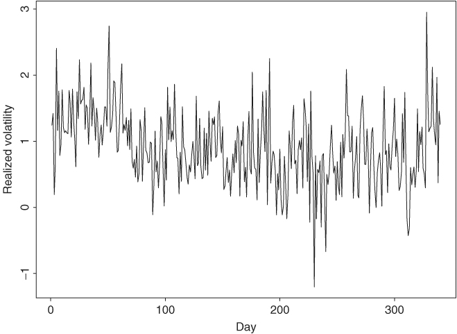
To illustrate the ideas of the state-space model and Kalman filter, we consider the intradaily realized volatility of Alcoa stock from January 2, 2003, to May 7, 2004, for 340 observations. The daily realized volatility used is the sum of squares of intraday 10-minute log returns measured in percentage. No overnight returns or the first 10-minute intraday returns are used. See Chapter 3 for more information about realized volatility. The series used in the demonstration is the logarithm of the daily realized volatility.
Figure 11.1 shows the time plot of the logarithms of the realized volatility of Alcoa stock from January 2, 2003, to May 7, 2004. The transactions data are obtained from the TAQ database of the NYSE. If ARIMA models are entertained, we obtain an ARIMA(0,1,1) model
where yt is the log realized volatility, and the standard error of ![]() is 0.028. The residuals show Q(12) = 12.4 with a p value of 0.33, indicating that there is no significant serial correlation in the residuals. Similarly, the squared residuals give Q(12) = 8.2 with a p value of 0.77, suggesting no ARCH effects in the series.
is 0.028. The residuals show Q(12) = 12.4 with a p value of 0.33, indicating that there is no significant serial correlation in the residuals. Similarly, the squared residuals give Q(12) = 8.2 with a p value of 0.77, suggesting no ARCH effects in the series.
Figure 11.1 Time plot of logarithms of intradaily realized volatility of Alcoa stock from January 2, 2003, to May 7, 2004. Realized volatility is computed from intraday 10-minute log returns measured in percentage.
Since ![]() is positive, we can transform the ARIMA(0,1,1) model into a local trend model in Eqs. (11.1) and (11.2). The maximum-likelihood estimates (MLE) of the two parameters are
is positive, we can transform the ARIMA(0,1,1) model into a local trend model in Eqs. (11.1) and (11.2). The maximum-likelihood estimates (MLE) of the two parameters are ![]() and
and ![]() . The measurement errors have a larger variance than the state innovations, confirming that intraday high-frequency returns are subject to measurement errors. Details of estimation will be discussed in Section 11.1.8. Here we treat the two estimates as given and use the model to demonstrate application of the Kalman filter. Note that using the model in Eq. (11.6) and the relation in Eqs. (11.4) and (11.5), we obtain σe = 0.480 and ση = 0.0736. These values are close to the MLE shown above.
. The measurement errors have a larger variance than the state innovations, confirming that intraday high-frequency returns are subject to measurement errors. Details of estimation will be discussed in Section 11.1.8. Here we treat the two estimates as given and use the model to demonstrate application of the Kalman filter. Note that using the model in Eq. (11.6) and the relation in Eqs. (11.4) and (11.5), we obtain σe = 0.480 and ση = 0.0736. These values are close to the MLE shown above.
11.1.2 Statistical Inference
Return to the state-space model in Eqs. (11.1) and (11.2). The aim of the analysis is to infer properties of the state μt from the data {yt|t = 1, … , T} and the model. Three types of inference are commonly discussed in the literature. They are filtering, prediction, and smoothing. Let Ft = {y1, … , yt} be the information available at time t (inclusive) and assume that the model is known, including all parameters. The three types of inference can briefly be described as follows:
- Filtering. Filtering means to recover the state variable μt given Ft, that is, to remove the measurement errors from the data.
- Prediction. Prediction means to forecast μt+h or yt+h for h > 0 given Ft, where t is the forecast origin.
- Smoothing. Smoothing is to estimate μt given FT, where T > t.
A simple analogy of the three types of inference is reading a handwritten note. Filtering is figuring out the word you are reading based on knowledge accumulated from the beginning of the note, predicting is to guess the next word, and smoothing is deciphering a particular word once you have read through the note.
To describe the inference more precisely, we introduce some notation. Let μt|j = E(μt|Fj) and Σt|j = Var(μt|Fj) be, respectively, the conditional mean and variance of μt given Fj. Similarly, yt|j denotes the conditional mean of yt given Fj. Furthermore, let vt = yt − yt|t−1 and Vt = Var(vt|Ft−1) be the 1-step-ahead forecast error and its variance of yt given Ft−1. Note that the forecast error vt is independent of Ft−1 so that the conditional variance is the same as the unconditional variance; that is, Var(vt|Ft−1) = Var(vt). From Eq. (11.1),
![]()
Consequently,
and
It is also easy to see that
![]()
Thus, as expected, the 1-step-ahead forecast error is uncorrelated (hence, independent) with yj for j < t. Furthermore, for the linear model in Eqs. (11.1) and (11.2), μt|t = E(μt|Ft) = E(μt|Ft−1, vt) and Σt|t = Var(μt|Ft) = Var(μt|Ft−1, vt). In other words, the information set Ft can be written as Ft = {Ft−1, yt} = {Ft−1, vt}.
The following properties of multivariate normal distribution are useful in studying the Kalman filter under normality. They can be shown via the multivariate linear regression method or factorization of the joint density. See, also, Appendix B of Chapter 8. For random vectors w and m, denote the mean vectors and covariance matrix as E(w)=μm, μm, and Cov(m, w)=Σmw, respectively.
Theorm 11.1.
Suppose that x, y, and z are three random vectors such that their joint distribution is multivariate normal. In addition, assume that the diagonal block covariance matrix Σww is nonsingular for w = x, y, z, and Σyz = 0. Then,
![]()
![]()
![]()
![]()
11.1.3 Kalman Filter
The goal of the Kalman filter is to update knowledge of the state variable recursively when a new data point becomes available. That is, knowing the conditional distribution of μt given Ft−1 and the new data yt, we would like to obtain the conditional distribution of μt given Ft, where, as before, Fj = {y1, … , yj}. Since Ft = {Ft−1, vt}, giving yt and Ft−1 is equivalent to giving vt and Ft−1. Consequently, to derive the Kalman filter, it suffices to consider the joint conditional distribution of (μt, vt)′ given Ft−1 before applying Theorem 11.1.
The conditional distribution of vt given Ft−1 is normal with mean zero and variance given in Eq. (11.8), and that of μt given Ft−1 is also normal with mean μt|t−1 and variance Σt|t−1. Furthermore, the joint distribution of (μt, vt)′ given Ft−1 is also normal. Thus, what remains to be solved is the conditional covariance between μt and vt given Ft−1. From the definition,
11.9 
where we have used the fact that E[μt|t−1(μt − μt|t−1)|Ft−1] = 0. Putting the results together, we have
![]()
By Theorem 11.1, the conditional distribution of μt given Ft is normal with mean and variance
11.11 ![]()
where Kt = Σt|t−1/Vt is commonly referred to as the Kalman gain, which is the regression coefficient of μt on vt. From Eq. (11.10), Kalman gain is the factor that governs the contribution of the new shock vt to the state variable μt.
Next, one can make use of the knowledge of μt given Ft to predict μt+1 via Eq. (11.2). Specifically, we have
11.12 ![]()
Once the new data yt+1 is observed, one can repeat the above procedure to update knowledge of μt+1. This is the famous Kalman filter algorithm proposed by Kalman (1960).
In summary, putting Eqs. (11.7) and (11.13) together and conditioning on the initial assumption that μ1 is distributed as N(μ1|0, Σ1|0), the Kalman filter for the local trend model is as follows:

There are many ways to derive the Kalman filter. We use Theorem 11.1, which describes some properties of multivariate normal distribution, for its simplicity. In practice, the choice of initial values Σ1|0 and μ1|0 requires some attention and we shall discuss it later in Section 11.1.7. For the local trend model in Eqs. (11.1) and (11.2), the two parameters σe and ση can be estimated via the maximum-likelihood method. Again, the Kalman filter is useful in evaluating the likelihood function of the data in estimation. We shall discuss estimation in Section 11.1.8.
Example 11.1 (Continued)
To illustrate application of the Kalman filter, we use the fitted state-space model for daily realized volatility of Alcoa stock returns and apply the Kalman filter algorithm to the data with Σ1|0 = ∞ and μ1|0 = 0. The choice of these initial values will be discussed in Section 11.1.7. Figure 11.2(a) shows the time plot of the filtered state variable μt|t, and Figure 11.2(b) is the time plot of the 1-step-ahead forecast error vt. Compared with Figure 11.1, the filtered states are smoother. The forecast errors appear to be stable and center around zero. These forecast errors are out-of-sample 1-step-ahead prediction errors.
Figure 11.2 Time plots of output of Kalman filter applied to daily realized log volatility of Alcoa stock based on local trend state-space model: (a) filtered state μt|t and (b) 1-step-ahead forecast error vt.

11.1.4 Properties of Forecast Error
The 1-step-ahead forecast errors {vt} are useful in many applications, hence it pays to study carefully their properties. Given the initial values Σ1|0 and μ1|0, which are independent of yt, the Kalman filter enables us to compute vt recursively as a linear function of {y1, … , yt}. Specifically, by repeated substitutions,

and so on. This transformation can be written in matrix form as
where v=(v1, … vT)′, y=(y1, … yT)′, is the T-dimensional vector of ones, and K is a lower triangular matrix defined as
where ki, i−1 = − Ki−1 and kij = − (1 − Ki−1)(1 − Ki−2) ⋯ (1 − Kj+1)Kj for i = 2, … , T and j = 1, … , i − 2. It should be noted that, from the definition, the Kalman gain Kt does not depend on μ1|0 or the data {y1, … , yt}; it depends on Σ1|0 and ![]() and
and ![]() .
.
The transformation in Eq. (11.5) has several important implications. First, {vt} are mutually independent under the normality assumption. To show this, consider the joint probability density function of the data
![]()
Equation (11.15) indicates that the transformation from yt to vt has a unit Jacobian so that p(v) = p(y). Furthermore, since μ1|0 is given, p(v1) = p(y1). Consequently, the joint probability density function of v is
![]()
This shows that {vt} are mutually independent.
Second, the Kalman filter provides a Cholesky decomposition of the covariance matrix of y. To see this, let = Cov(y). Equation (11.15) shows that Cov(v) = K K′. On the other hand, {vt} are mutually independent with Var(vt) = Vt. Therefore, K K′ = diag{V1, … ,VT}, which is precisely a Cholesky decomposition of . The elements kij of the matrix K thus have some nice interpretations; see Chapter 10.
State Error Recursion
Turn to the estimation error of the state variable μt. Define
![]()
as the forecast error of the state variable μt given data Ft−1. From Section 11.1.711.1.1, Var(xt|Ft−1) = Σt|t−1. From the Kalman filter in Eq. (11.14),
![]()
and
![]()
where ![]() . Consequently, for the state errors, we have
. Consequently, for the state errors, we have
where x1 = μ1 − μ1|0. Equation (11.16) is in the form of a time-varying state-space model with xt being the state variable and vt the observation.
11.1.5 State Smoothing
Next we consider the estimation of the state variables {μ1, … , μT} given the data FT and the model. That is, given the state-space model in Eqs. (11.1) and (11.2), we wish to obtain the conditional distribution μt|FT for all t. To this end, we first recall some facts available about the model:
- All distributions involved are normal so that we can write the conditional distribution of μt given FT as N(μt|T, Σt|T), where t ≤ T. We refer to μt|T as the smoothed state at time t and Σt|T as the smoothed state variance.
- Based on the properties of {vt} shown in Section 11.1.4, {v1, … , vT} are mutually independent and are linear functions of {y1, … , yT}.
- If y1, … , yT are fixed, then Ft−1 and {vt, … , vT} are fixed, and vice versa.
- {vt, … , vT} are independent of Ft−1 with mean zero and variance Var(vj) = Vj for j ≥ t.
Applying Theorem 11.1(3) to the conditional joint distribution of (μt, vt, … , vT) given Ft−1, we have
From the definition and independence of {vt}, Cov(μt, vj) = Cov(xt, vj) for j = t, … , T, and
![]()
Similarly, we have

Consequently, Eq. (11.17) becomes

where

is a weighted linear combination of the innovations {vt, … , vT}. This weighted sum satisfies
Therefore, using the initial value qT = 0, we have the backward recursion
Putting Eqs. (11.17) and (11.19) together, we have a backward recursive algorithm to compute the smoothed state variables:
where qT = 0, and μt|t−1, Σt|t−1 and Lt are available from the Kalman filter in Eq. (11.14).
Smoothed State Variance
The variance of the smoothed state variable μt|T can be derived in a similar manner via Theorem 11.1(4). Specifically, letting ![]() , we have
, we have
11.21 
where Cov(μt, vj) = Cov(xt, vj) are given earlier after Eq. (11.17). Thus,
11.22 
where

is a weighted linear combination of the inverses of variances of the 1-step-ahead forecast errors after time t − 1. Let MT = 0 because no 1-step-ahead forecast error is available after time index T. The statistic Mt−1 can be written as

Note that from the independence of {vt} and Eq. (11.18), we have

Combining the results, variances of the smoothed state variables can be computed efficiently via the backward recursion
where MT = 0.
Example
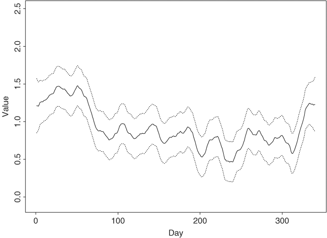
Example 11.1 (Continued)Applying the Kalman filter and state-smoothing algorithms in Eqs. (11.20) and (11.23) to the daily realized volatility of Alcoa stock using the fitted state-space model, we can easily compute the filtered state μt|t and the smoothed state μt|T and their variances. Figure 11.3 shows the filtered state variable and its 95% pointwise confidence interval, whereas Figure 11.4 provides the time plot of smoothed state variable and its 95% pointwise confidence interval. As expected, the smoothed state variables are smoother than the filtered state variables. The confidence intervals for the smoothed state variables are also narrower than those of the filtered state variables. Note that the width of the 95% confidence interval of μ1|1 depends on the initial value Σ1|0.
Figure 11.3 Filtered state variable μt|t and its 95% pointwise confidence interval for daily log realized volatility of Alcoa stock returns based on fitted local-trend state-space model.

Figure 11.4 Smoothed state variable μt|T and its 95% pointwise confidence interval for daily log realized volatility of Alcoa stock returns based on fitted local-trend state-space model.
11.1.6 Missing Values
An advantage of the state-space model is in handling missing values. Suppose that the observations ![]() are missing, where h ≥ 1 and 1 ≤ ℓ < T. There are several ways to handle missing values in state-space formulation. Here we discuss a method that keeps the original time scale and model form. For t ∈ {ℓ + 1, … , ℓ + h}, we can use Eq. (11.2) to express μt as a linear combination of μℓ+1 and
are missing, where h ≥ 1 and 1 ≤ ℓ < T. There are several ways to handle missing values in state-space formulation. Here we discuss a method that keeps the original time scale and model form. For t ∈ {ℓ + 1, … , ℓ + h}, we can use Eq. (11.2) to express μt as a linear combination of μℓ+1 and ![]() . Specifically,
. Specifically,
![]()
where it is understood that the summation term is zero if its lower limit is greater than its upper limit. Therefore, for t ∈ {ℓ + 1, … , ℓ + h},
![]()
Consequently, we have
11.24 ![]()
for t = ℓ + 2, … , ℓ + h. These results show that we can continue to apply the Kalman filter algorithm in Eq. (11.14) by taking vt = 0 and Kt = 0 for t = ℓ + 1, … , ℓ + h. This is rather natural because when yt is missing, there is no new innovation or new Kalman gain so that vt = 0 and Kt = 0.
11.1.7 Effect of Initialization
In this section, we consider the effects of initial condition μ1 ∼ N(μ1|0, Σ1|0) on the Kalman filter and state smoothing. From the Kalman filter in Eq. (11.14),
![]()
and, by Eqs. (11.10)–(11.13),
Therefore, letting Σ1|0 increase to infinity, we have μ2|1 = y1 and ![]() . This is equivalent to treating y1 as fixed and assuming
. This is equivalent to treating y1 as fixed and assuming ![]() . In the literature, this approach to initializing the Kalman filter is called diffuse initialization because a very large Σ1|0 means one is uncertain about the initial condition.
. In the literature, this approach to initializing the Kalman filter is called diffuse initialization because a very large Σ1|0 means one is uncertain about the initial condition.
Next, turn to the effect of diffuse initialization on state smoothing. It is obvious that based on the results of Kalman filtering, state smoothing is not affected by the diffuse initialization for t = T, … , 2. Thus, we focus on μ1 given FT. From Eq. (11.20) and the definition of ![]() ,
,
Letting Σ1|0 → ∞, we have ![]() . Furthermore, from Eq. (11.23) and using
. Furthermore, from Eq. (11.23) and using ![]() , we have
, we have
Thus, letting Σ1|0 → ∞, we obtain ![]() .
.
Based on the prior discussion, we suggest using diffuse initialization when little is known about the initial value μ1. However, it might be hard to justify the use of a random variable with infinite variance in real applications. If necessary, one can treat μ1 as an additional parameter of the state-space model and estimate it jointly with other parameters. This latter approach is closely related to the exact maximum-likelihood estimation of Chapters 2 and 8.
11.1.8 Estimation
In this section, we consider the estimation of σe and ση of the local trend model in Eqs. (11.1) and (11.2). Based on properties of forecast errors discussed in Section 11.1.4, the Kalman filter provides an efficient way to evaluate the likelihood function of the data for estimation. Specifically, the likelihood function under normality is

where y1 ∼ N(μ1|0, V1) and vt = (yt − μt|t−1) ∼ N(0, Vt). Consequently, assuming μ1|0 and Σ1|0 are known, and taking the logarithms, we have
11.25 ![]()
which involves vt and Vt. Therefore, the log-likelihood function, including cases with missing values, can be evaluated recursively via the Kalman filter. Many software packages perform state-space model estimation via a Kalman filter algorithm such as Matlab, RATS, and S-Plus. In this chapter, we use the SsfPack program developed by Koopman, Shephard, and Doornik (1999) and available in S-Plus and OX. Both Ssfpack and OX are free and can be downloaded from their websites.
11.1.9 S-Plus Commands Used
We provide here the SsfPack commands used to perform analysis of the daily realized volatility of Aloca stock returns. Only brief explanations are given. For further details of the commands used, see Durbin and Koopman (2001, Section 6.5). S-Plus uses specific notation to specify a state-space model; see Table 11.1. The notation must be followed closely. In Table 11.2, we give some commands and their functions.
Table 11.1 State-Space Form and Notation in S-Plus
| State-Space Parameter | S-Plus Name |
| δ | mDelta |
| Φ | mPhi |
| Ω | mOmega |
| Σ | mSigma |
Table 11.2 Some Commands of SsfPack Package
| Command | Function |
| SsfFit | Maximum-likelihood estimation |
| CheckSsf | Create “Ssf” object in S-Plus |
| KalmanFil | Perform Kalman filtering |
| KalmanSmo | Perform state smoothing |
| SsfMomentEst with task “STFIL” | Compute filtered state and variance |
| SsfMomentEst with task “STSMO” | Compute smoothed state and variance |
| SsfCondDens with task “STSMO” | Compute smoothed state without variance |
In our analysis, we first perform maximum-likelihood estimation of the state-space model in Eqs. (11.1) and (11.2) to obtain estimates of σe and ση. The initial values used are Σ1|0 = − 1 and μ1|0 = 0, where − 1 signifies diffuse initialization, that is, Σ1|0 is very large. We then treat the fitted model as given to perform Kalman filtering and state smoothing.
SsfPack and S-Plus Commands for State-Space Model
> da = read.table(file='aa-rv-0304.txt',header=F) % load data
> y = log(da[,1]) % log(RV)
> ltm.start=c(3,1) % Initial parameter values
> P1 = -1 % Initialization of Kalman filter
> a1 = 0
> ltm.m=function(parm){ % Specify a function for the
+ sigma.eta=parm[1] % local trend model.
+ sigma.e=parm[2]
+ ssf.m=list(mPhi=as.matrix(c(1,1)),
+ mOmega=diag(c(sigma.eta^2,sigma.e^2)),
+ mSigma=as.matrix(c(P1,a1)))
+ CheckSsf(ssf.m)
+ }
% perform estimation
> ltm.mle=SsfFit(ltm.start,y,"ltm.m",lower=c(0,0),
+ upper=c(100,100))
> ltm.mle$parameters
[1] 0.07350827 0.48026284
> sigma.eta=ltm.mle$parameters[1]
> sigma.eta
[1] 0.07350827
> sigma.e=ltm.mle$parameters[2]
> sigma.e
[1] 0.4802628
% Specify a state-space model in S-Plus.
> ssf.ltm.list=list(mPhi=as.matrix(c(1,1)),
+ mOmega=diag(c(sigma.eta^2,sigma.e^2)),
+ mSigma=as.matrix(c(P1,a1)))
% check validity of the specified model.
> ssf.ltm=CheckSsf(ssf.ltm.list)
> ssf.ltm
$mPhi:
[,1]
[1,] 1
[2,] 1
$mOmega:
[,1] [,2]
[1,] 0.0054035 0.0000000
[2,] 0.0000000 0.2306524
$mSigma:
[,1]
[1,] -1
[2,] 0
$mDelta:
[,1]
[1,] 0
[2,] 0
$mJPhi:
[1] 0
$mJOmega:
[1] 0
$mJDelta:
[1] 0
$mX:
[1] 0
$cT:
[1] 0
$cX:
[1] 0
$cY:
[1] 1
$cSt:
[1] 1
attr(, "class"):
[1] "ssf"
% Apply Kalman filter
> KalmanFil.ltm=KalmanFil(y,ssf.ltm,task="STFIL")
> names(KalmanFil.ltm)
[1] "mOut" "innov" "std.innov" "mGain" "loglike"
[6] "loglike.conc" "dVar" "mEst" "mOffP" "task"
[11] "err" "call"
> par(mfcol=c(2,1)) % Obtain plot
> plot(KalmanFil.ltm$ mEst[,1],xlab='day',
+ ylab='filtered state',type='l')
> title(main='(a) Filtered state variable')
> plot(KalmanFil.ltm$ mOut[,1],xlab='day',
+ ylab='v(t)',type='l')
> title(main='(b) Prediction error')
% Obtain residuals and their variances
> KalmanSmo.ltm=KalmanSmo(KalmanFil.ltm,ssf.ltm)
> names(KalmanSmo.ltm)
[1] "state.residuals" "response.residuals" "state.variance"
[4] "response.variance" "aux.residuals" "scores"
[7] "call"
% Filtered states
> FiledEst.ltm=SsfMomentEst(y,ssf.ltm,task="STFIL")
> names(FiledEst.ltm)
[1] "state.moment" "state.variance" "response.moment"
[4] "response.variance" "task"
% Smoothed states
> SmoedEst.ltm=SsfMomentEst(y,ssf.ltm,task="STSMO")
> names(SmoedEst.ltm)
[1] "state.moment" "state.variance" "response.moment"
[4] "response.variance" "task"
% Obtain plots of filtered and smoothed states with 95% C.I.
> up=FiledEst.ltm$ state.moment+
+ 2*sqrt(FiledEst.ltm$ state.variance)
> lw=FiledEst.ltm$ state.moment-
+ 2*sqrt(FiledEst.ltm$ state.variance)
> par(mfcol=c(1,1))
> plot(FiledEst.ltm$ state.moment,type='l',xlab='day',
+ ylab='value',ylim=c(-0.1,2.5))
> lines(1:340,up,lty=2)
> lines(1:340,lw,lty=2)
> title(main='Filed state variable')
> up=SmoedEst.ltm$ state.moment+
+ 2*sqrt(SmoedEst.ltm$ state.variance)
> lw=SmoedEst.ltm$ state.moment-
+ 2*sqrt(SmoedEst.ltm$ state.variance)
> plot(SmoedEst.ltm$ state.moment,type='l',xlab='day',
+ ylab='value',ylim=c(-0.1,2.5))
> lines(1:340,up,lty=2)
> lines(1:340,lw,lty=2)
> title(main='Smoothed state variable')
% Model checking via standardized residuals
> resi=KalmanFil.ltm$ mOut[,1]*sqrt(KalmanFil.ltm$ mOut[,3])
> archTest(resi)
> autocorTest(resi)
For the daily realized volatility of Alcoa stock returns, the fitted local trend model is adequate based on residual analysis. Specifically, given the parameter estimates, we use the Kalman filter to obtain the 1-step-ahead forecast error vt and its variance Vt. We then compute the standardized forecast error ![]() and check the serial correlations and ARCH effects of
and check the serial correlations and ARCH effects of ![]() . We found that Q(25) = 23.37(0.56) for the standardized forecast errors, and the LM test statistic for ARCH effect is 18.48(0.82) for 25 lags, where the number in parentheses denotes p value.
. We found that Q(25) = 23.37(0.56) for the standardized forecast errors, and the LM test statistic for ARCH effect is 18.48(0.82) for 25 lags, where the number in parentheses denotes p value.