7.5 Extreme Value Theory

In this section, we review some extreme value theory in the statistical literature. Denote the return of an asset, measured in a fixed time interval such as daily, by rt. Consider the collection of n returns, {r1, … , rn}. The minimum return of the collection is r(1), that is, the smallest order statistic, whereas the maximum return is r(n), the maximum order statistic. Specifically, r(1) = min1≤j≤n{rj} and r(n) = max1≤j≤n{rj}. Following the literature and using the loss function in VaR calculation, we focus on properties of the maximum return r(n). However, the theory discussed also applies to the minimum return of an asset over a given time period because properties of the minimum return can be obtained from those of the maximum by a simple sign change. Specifically, we have , where with the superscript c denoting sign change. The minimum return is relevant to holding a long financial position. As before, we shall use negative log returns, instead of the log returns, to perform VaR calculation for a long position.

7.5.1 Review of Extreme Value Theory

Assume that the returns rt are serially independent with a common cumulative distribution function F(x) and that the range of the return rt is [l, u]. For log returns, we have . Then the CDF of r(n), denoted by Fn, n(x), is given by

7.15

In practice, the CDF F(x) of rt is unknown and, hence, Fn, n(x) of r(n) is unknown. However, as n increases to infinity, Fn, n(x) becomes degenerated—namely, Fn, n(x) → 0 if x < u and Fn, n(x) → 1 if x ≥ u as n goes to infinity. This degenerated CDF has no practical value. Therefore, the extreme value theory is concerned with finding two sequences {βn} and {αn}, where αn > 0, such that the distribution of r(n*) ≡ (r(n) − βn)/αn converges to a nondegenerate distribution as n goes to infinity. The sequence {βn} is a location series and {αn} is a series of scaling factors. Under the independent assumption, the limiting distribution of the normalized minimum r(n*) is given by

7.16

for x < − 1/ξ if ξ < 0 and for x > − 1/ξ if ξ > 0, where the subscript * signifies the maximum. The case of ξ = 0 is taken as the limit when ξ → 0. The parameter ξ is referred to as the shape parameter that governs the tail behavior of the limiting distribution. The parameter α = 1/ξ is called the tail index of the distribution.

The limiting distribution in Eq. (7.16) is the generalized extreme value (GEV) distribution of Jenkinson (1955) for the maximum. It encompasses the three types of limiting distribution of Gnedenko (1943):

• Type I: ξ = 0, the Gumbel family. The CDF is

7.17

• Type II: ξ > 0, the Fréchet family. The CDF is

7.18

• Type III: ξ < 0, the Weibull family. The CDF here is

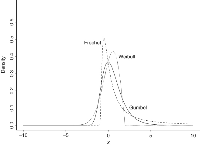
Gnedenko (1943) gave necessary and sufficient conditions for the CDF F(x) of rt to be associated with one of the three types of limiting distribution. Briefly speaking, the tail behavior of F(x) determines the limiting distribution F*(x) of the maximum. The right tail of the distribution declines exponentially for the Gumbel family, by a power function for the Fréchet family, and is finite for the Weibull family (Figure 7.2). Readers are referred to Embrechts, Kuppelberg, and Mikosch (1997) for a comprehensive treatment of the extreme value theory. For risk management, we are mainly interested in the Fréchet family, which includes stable and Student-t distributions. The Gumbel family consists of thin-tailed distributions such as normal and lognormal distributions. The probability density function (pdf) of the generalized limiting distribution in Eq. (7.16) can be obtained easily by differentiation:

7.19

where for ξ = 0, and x < − 1/ξ for ξ < 0, and x > − 1/ξ for ξ > 0.

Figure 7.2 Probability density functions of extreme value distributions for maximum. Solid line is for Gumbel distribution, dotted line is for Weibull distribution with ξ = − 0.5, and dashed line is for Fréchet distribution with ξ = 0.9.

The aforementioned extreme value theory has two important implications. First, the tail behavior of the CDF F(x) of rt, not the specific distribution, determines the limiting distribution F*(x) of the (normalized) maximum. Thus, the theory is generally applicable to a wide range of distributions for the return rt. The sequences {βn} and {αn}, however, may depend on the CDF F(x). Second, Feller (1971, p. 279) shows that the tail index ξ does not depend on the time interval of rt. That is, the tail index (or equivalently the shape parameter) is invariant under time aggregation. This second feature of the limiting distribution becomes handy in the VaR calculation.

The extreme value theory has been extended to serially dependent observations provided that the dependence is weak. Berman (1964) shows that the same form of the limiting extreme value distribution holds for stationary normal sequences provided that the autocorrelation function of rt is squared summable (i.e., ), where ρi is the lag-i autocorrelation function of rt. For further results concerning the effect of serial dependence on the extreme value theory, readers are referred to Leadbetter, Lindgren, and Rootzén (1983, Chapter 3). We shall discuss extremal index for a strictly stationary time series later in Section 7.8.

7.5.2 Empirical Estimation

The extreme value distribution contains three parameters—ξ, βn, and αn. These parameters are referred to as the shape, location, and scale parameters, respectively. They can be estimated by using either parametric or nonparametric methods. We review some of the estimation methods.

For a given sample, there is only a single minimum or maximum, and we cannot estimate the three parameters with only an extreme observation. Alternative ideas must be used. One of the ideas used in the literature is to divide the sample into subsamples and apply the extreme value theory to the subsamples. Assume that there are T returns available. We divide the sample into g nonoverlapping subsamples each with n observations, assuming for simplicity that T = ng. In other words, we divide the data as

and write the observed returns as rin+j, where 1 ≤ j ≤ n and i = 0, … , g − 1. Note that each subsample corresponds to a subperiod of the data span. When n is sufficiently large, we hope that the extreme value theory applies to each subsample. In application, the choice of n can be guided by practical considerations. For example, for daily returns, n = 21 corresponds approximately to the number of trading days in a month and n = 63 denotes the number of trading days in a quarter.

Let rn, i be the maximum of the ith subsample (i.e., rn, i is the largest return of the ith subsample), where the subscript n is used to denote the size of the subsample. When n is sufficiently large, xn, i = (rn, i − βn)/αn should follow an extreme value distribution, and the collection of subsample maxima {rn, i|i = 1, … , g} can then be regarded as a sample of g observations from that extreme value distribution. Specifically, we define

7.20

The collection of subsample maxima {rn, i} is the data we use to estimate the unknown parameters of the extreme value distribution. Clearly, the estimates obtained may depend on the choice of subperiod length n.

7.5.2.1 The Parametric Approach

Two parametric approaches are available. They are the maximum-likelihood and regression methods.

7.5.2.2 Maximum-Likelihood Method

Assuming that the subperiod maxima {rn, i} follow a generalized extreme value distribution such that the pdf of xi = (rn, i − βn)/αn is given in Eq. (7.19), we can obtain the pdf of rn, i by a simple transformation as

where it is understood that 1 + ξn(rn, i − βn)/αn > 0 if ξn ≠ 0. The subscript n is added to the shape parameter ξ to signify that its estimate depends on the choice of n. Under the independence assumption, the likelihood function of the subperiod maxima is

Nonlinear estimation procedures can then be used to obtain maximum-likelihood estimates of ξn, βn, and αn. These estimates are unbiased, asymptotically normal, and of minimum variance under proper assumptions. See Embrechts et al. (1997) and Coles (2001) for details. We apply this approach to some stock return series later.

7.5.2.3 Regression Method

This method assumes that is a random sample from the generalized extreme value distribution in Eq. (7.16) and makes use of properties of order statistics; see Gumbel (1958). Denote the order statistics of the subperiod maxima as

Using properties of order statistics (e.g., Cox and Hinkley, 1974, p. 467), we have

7.21

For simplicity, we separate the discussion into two cases depending on the value of ξ. First, consider the case of ξ ≠ 0. From Eq. (7.16), we have

7.22

Consequently, using Eqs. (7.21) and (7.22) and approximating expectation by an observed value, we have

Taking natural logarithm twice, the prior equation gives

In practice, letting ei be the deviation between the previous two quantities and assuming that the series {et} is not serially correlated, we have a regression setup

7.23

The least-squares estimates of ξn, βn, and αn can be obtained by minimizing the sum of squares of ei.

When ξn = 0, the regression setup reduces to

The least-squares estimates are consistent but less efficient than the likelihood estimates. We use the likelihood estimates in this chapter.

7.5.2.4 The Nonparametric Approach

The shape parameter ξ can be estimated using some nonparametric methods. We mention two such methods here. These two methods are proposed by Hill (1975) and Pickands (1975) and are referred to as the Hill estimator and Pickands estimator, respectively. Both estimators apply directly to the returns . Thus, there is no need to consider subsamples. Denote the order statistics of the sample as

Let q be a positive integer. The two estimators of ξ are defined as

7.24

7.25

where the argument (q) is used to emphasize that the estimators depend on q and the subscripts p and h denote Pickands and Hill estimators, respectively. The choice of q differs between Hill and Pickands estimators. It has been investigated by several researchers, but there is no general consensus on the best choice available. Dekkers and De Haan (1989) show that ξp(q) is consistent if q increases at a properly chosen pace with the sample size T. In addition, is asymptotically normal with mean zero and variance ξ2(22ξ+1 + 1)/[2(2ξ − 1)ln(2)]2. The Hill estimator is applicable to the Fréchet distribution only, but it is more efficient than the Pickands estimator when applicable. Goldie and Smith (1987) show that is asymptotically normal with mean zero and variance ξ2. In practice, one may plot the Hill estimator ξh(q) against q and find a proper q such that the estimate appears to be stable. The estimated tail index α = 1/ξh(q) can then be used to obtain extreme quantiles of the return series; see Zivot and Wang (2003).

7.5.3 Application to Stock Returns

We apply the extreme value theory to the daily log returns of IBM stock from July 3, 1962, to December 31, 1998. The returns are measured in percentages, and the sample size is 9190 (i.e., T = 9190). Figure 7.3 shows the time plots of extreme daily log returns when the length of the subperiod is 21 days, which corresponds approximately to a month. The October 1987 crash is clearly seen from the plot. Excluding the 1987 crash, the range of extreme daily log returns is between 0.5 and 13%.

Figure 7.3 Maximum and minimum daily log returns of IBM stock when subperiod is 21 trading days. Data span is from July 3, 1962, to December 31, 1998: (a) positive returns and (b) negative returns.

Table 7.1 summarizes some estimation results of the shape parameter ξ via the Hill estimator. Three choices of q are reported in the table, and the results are stable. To provide an overall picture of the performance of the Hill estimator, Figure 7.4 shows the scatterplots of the Hill estimator ξh(q) and its pointwise 95% confidence interval against q. For both positive and negative extreme daily log returns, the estimator is stable except for cases when q is small. The estimated shape parameters are about 0.30 and are significantly different from zero at the asymptotic 5% level. The plots also indicate that the shape parameter ξ appears to be larger for the negative extremes, indicating that the daily log return may have a heavier left tail. Overall, the result indicates that the distribution of daily log returns of IBM stock belongs to the Fréchet family. The analysis thus rejects the normality assumption commonly used in practice. Such a conclusion is in agreement with that of Longin (1996), who used a U.S. stock market index series. R and S-Plus commands used to perform the analysis are given in the demonstration below.

Figure 7.4 Scatterplots of Hill estimator for daily log returns of IBM stock. Sample period is from July 3, 1962, to December 31, 1998: upper plot is for positive returns and lower one for negative returns.

Table 7.1 Results of Hill Estimator for Daily Log Returns of IBM Stock from July 3, 1962, to December 31, 1998a

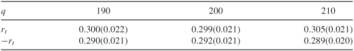
aStandard errors are in parentheses.

Next, we apply the maximum-likelihood method to estimate parameters of the generalized extreme value distribution for IBM daily log returns. Table 7.2 summarizes the estimation results for different choices of the length of subperiods ranging from 1 month (n = 21) to 1 year (n = 252). From the table, we make the following observations:

• Estimates of the location and scale parameters βn and αn increase in modulus as n increases. This is expected as magnitudes of the subperiod minimum and maximum are nondecreasing functions of n.
• Estimates of the shape parameter (or equivalently the tail index) are stable for the negative extremes when n ≥ 63 and are approximately 0.33.
• Estimates of the shape parameter are less stable for the positive extremes. The estimates are smaller in magnitude but remain significantly different from zero.
• The results for n = 252 have higher variabilities as the number of subperiods g is relatively small.

Again the conclusion obtained is similar to that of Longin (1996), who provided a good illustration of applying the extreme value theory to stock market returns.

Table 7.2 Maximum-Likelihood Estimates of Extreme Value Distribution for Daily Log Returns of IBM Stock from July 3, 1962 to December 31, 1998a

aStandard errors are in parentheses.

The results of Table 7.2 were obtained using a Fortran program developed by Richard Smith and modified by the author. The package evir of R performs similar estimation. S-Plus is also based on the evir package. I demonstrate below the commands used. Note that the package uses subgroup maxima in the estimation so that negative log returns are used for holding long financial positions. Furthermore, xi, sigma, mu in the package corresponds to (ξn, αn, βn) of the table. The estimates obtained by R and S-Plus are close to those in Table 7.2. A source of minor difference is that in Table 7.2 I dropped some data points at the beginning when the sample size T is not a multiple of the subgroup size n. Consequently, results of the R package have one more subgroup than that of Table 7.2.

7.5.3.1 R Demonstration for Extreme Value Analysis

The series is daily IBM log returns from 1962 to 1998. The following output was edited:

Define the residuals of a GEV distribution fit as

Using the pdf of the GEV distribution and transformation of variables, one can easily show that {wi} should form an iid random sample of exponentially distributed random variables if the fitted model is correctly specified. Figure 7.5 shows the residual plots of the GEV distribution fit to the daily negative IBM log returns with subperiod length of 21 days. The left panel gives the residuals and the right panel shows a quantile-to-quantile (QQ) plot against an exponential distribution. The plots indicate that the fit is reasonable.

Figure 7.5 Residual plots from fitting GEV distribution to daily negative IBM log returns, in percentage, for data from July 3, 1962, to December 31, 1998, with subperiod length of 21 days.