
7.6 Extreme Value Approach to VaR
In this section, we discuss an approach to VaR calculation using the extreme value theory. The approach is similar to that of Longin (1999a,b), who proposed an eight-step procedure for the same purpose. We divide the discussion into two parts. The first part is concerned with parameter estimation using the method discussed in the previous subsections. The second part focuses on VaR calculation by relating the probabilities of interest associated with different time intervals.
Part I
Assume that there are T observations of an asset return available in the sample period. We partition the sample period into g nonoverlapping subperiods of length n such that T = ng. If T = ng + m with 1 ≤ m < n, then we delete the first m observations from the sample. The extreme value theory discussed in the previous section enables us to obtain estimates of the location, scale, and shape parameters βn, αn, and ξn for the subperiod maxima {rn, i}. Plugging the maximum-likelihood estimates into the CDF in Eq. (7.16) with x = (r − βn)/αn, we can obtain the quantile of a given probability of the generalized extreme value distribution. Let p* be a small upper tail probability that indicates the potential loss and ![]() be the (1 − p*)th quantile of the subperiod maxima under the limiting generalized extreme value distribution. Then we have
be the (1 − p*)th quantile of the subperiod maxima under the limiting generalized extreme value distribution. Then we have
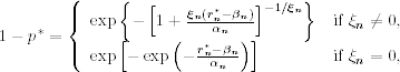
where it is understood that ![]() for ξn ≠ 0. Rewriting this equation as
for ξn ≠ 0. Rewriting this equation as
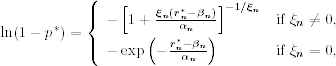
we obtain the quantile as
In financial applications, the case of ξn ≠ 0 is of major interest.
7.6.1.1 Part II
For a given upper tail probability p*, the quantile ![]() of Eq. (7.26) is the VaR based on the extreme value theory for the subperiod maximum. The next step is to make explicit the relationship between subperiod maxima and the observed return rt series.
of Eq. (7.26) is the VaR based on the extreme value theory for the subperiod maximum. The next step is to make explicit the relationship between subperiod maxima and the observed return rt series.
Because most asset returns are either serially uncorrelated or have weak serial correlations, we may use the relationship in Eq. (7.15) and obtain
This relationship between probabilities allows us to obtain VaR for the original asset return series rt. More precisely, for a specified small upper probability p, the (1 − p)th quantile of rt is ![]() if the upper tail probability p* of the subperiod maximum is chosen based on Eq. (7.27), where
if the upper tail probability p* of the subperiod maximum is chosen based on Eq. (7.27), where ![]() . Consequently, for a given small upper tail probability p, the VaR of a financial position with log return rt is
. Consequently, for a given small upper tail probability p, the VaR of a financial position with log return rt is
where n is the length of the subperiod.
7.6.1.2 Summary
We summarize the approach of applying the traditional extreme value theory to VaR calculation as follows:
1. Select the length of the subperiod n and obtain subperiod maxima {rn, i}, i = 1, … , g, where g = [T/n].
2. Obtain the maximum-likelihood estimates of βn, αn, and ξn.
3. Check the adequacy of the fitted extreme value model; see the next section for some methods of model checking.
4. If the extreme value model is adequate, apply Eq. (7.28) to calculate VaR.
Remark
Since we focus on loss function so that maxima of log returns are used in the derivation. Keep in mind that for a long financial position, the return series used in loss function is the negative log returns, not the traditional log returns. □
Example 7.6
Consider the daily log return, in percentage, of IBM stock from July 3, 1962, to December 31, 1998. From Table 7.2, we have ![]() ,
, ![]() , and
, and ![]() for n = 63. Therefore, for the left-tail probability p = 0.01, the corresponding VaR is
for n = 63. Therefore, for the left-tail probability p = 0.01, the corresponding VaR is
![]()
Thus, for daily negative log returns of the stock, the upper 1% quantile is 3.04969. If one holds a long position on the stock worth $10 million, then the estimated VaR with probability 1% is $10, 000, 000 × 0.0304969 = $304, 969. If the probability is 0.05, then the corresponding VaR is $166, 641.
If we chose n = 21 (i.e., approximately 1 month), then ![]() ,
, ![]() , and
, and ![]() . The upper 1% quantile of the negative log returns based on the extreme value distribution is
. The upper 1% quantile of the negative log returns based on the extreme value distribution is
![]()
Therefore, for a long position of $10, 000, 000, the corresponding 1-day horizon VaR is $340, 013 at the 1% risk level. If the probability is 0.05, then the corresponding VaR is $184, 127. In this particular case, the choice of n = 21 gives higher VaR values.
It is somewhat surprising to see that the VaR values obtained in Example 7.6 using the extreme value theory are smaller than those of Example 7.3 that uses a GARCH(1,1) model. In fact, the VaR values of Example 7.6 are even smaller than those based on the empirical quantile in Example 7.5. This is due in part to the choice of probability 0.05. If one chooses probability 0.001 = 0.1% and considers the same financial position, then we have VaR = $546, 641 for the Gaussian AR(2)–GARCH(1,1) model and VaR = $666, 590 for the extreme value theory with n = 21. Furthermore, the VaR obtained here via the traditional extreme value theory may not be adequate because the independent assumption of daily log returns is often rejected by statistical testings. Finally, the use of subperiod maxima overlooks the fact of volatility clustering in the daily log returns. The new approach of extreme value theory discussed in the next section overcomes these weaknesses.
Remark
As shown by the results of Example 7.6, the VaR calculation based on the traditional extreme value theory depends on the choice of n, which is the length of subperiods. For the limiting extreme value distribution to hold, one would prefer a large n. But a larger n means a smaller g when the sample size T is fixed, where g is the effective sample size used in estimating the three parameters αn, βn, and ξn. Therefore, some compromise between the choices of n and g is needed. A proper choice may depend on the returns of the asset under study. We recommend that one should check the stability of the resulting VaR in applying the traditional extreme value theory. □
7.6.2 Discussion
We have applied various methods of VaR calculation to the daily log returns of IBM stock for a long position of $10 million. Consider the VaR of the position for the next trading day. If the probability is 5%, which means that with probability 0.95 the loss will be less than or equal to the VaR for the next trading day, then the results obtained are
1. $302, 500 for the RiskMetrics
2. $287, 200 for a Gaussian AR(2)–GARCH(1,1) model
3. $283, 520 for an AR(2)–GARCH(1,1) model with a standardized Student-t distribution with 5 degrees of freedom
4. $216, 030 for using the empirical quantile
5. $184, 127 for applying the traditional extreme value theory using monthly minima (i.e., subperiod length n = 21) of the log returns (or maxima of the negative log returns)
If the probability is 1%, then the VaR is
1. $426, 500 for the RiskMetrics
2. $409, 738 for a Gaussian AR(2)–GARCH(1,1) model
3. $475, 943 for an AR(2)–GARCH(1,1) model with a standardized Student-t distribution with 5 degrees of freedom
4. $365, 709 for using the empirical quantile
5. $340, 013 for applying the traditional extreme value theory using monthly minima (i.e., subperiod length n = 21)
If the probability is 0.1%, then the VaR becomes
1. $566, 443 for the RiskMetrics
2. $546, 641 for a Gaussian AR(2)–GARCH(1,1) model
3. $836, 341 for an AR(2)–GARCH(1,1) model with a standardized Student-t distribution with 5 degrees of freedom
4. $780, 712 for using the empirical quantile
5. $666, 590 for applying the traditional extreme value theory using monthly minima (i.e., subperiod length n = 21)
There are substantial differences among different approaches. This is not surprising because there exists substantial uncertainty in estimating tail behavior of a statistical distribution. Since there is no true VaR available to compare the accuracy of different approaches, we recommend that one applies several methods to gain insight into the range of VaR.
The choice of tail probability also plays an important role in VaR calculation. For the daily IBM stock returns, the sample size is 9190 so that the empirical quantiles of 5 and 1% are decent estimates of the quantiles of the return distribution. In this case, we can treat the results based on empirical quantiles as conservative estimates of the true VaR (i.e., lower bounds). In this view, the approach based on the traditional extreme value theory seems to underestimate the VaR for the daily log returns of IBM stock. The conditional approach of extreme value theory discussed in the next section overcomes this weakness.
When the tail probability is small (e.g., 0.1%), the empirical quantile is a less reliable estimate of the true quantile. The VaR based on empirical quantiles can no longer serve as a lower bound of the true VaR. Finally, the earlier results show clearly the effects of using a heavy-tail distribution in VaR calculation when the tail probability is small. The VaR based on either a Student-t distribution with 5 degrees of freedom or the extreme value distribution is greater than that based on the normal assumption when the probability is 0.1%.
7.6.3 Multiperiod VaR
The square root of time rule of the RiskMetrics methodology becomes a special case under the extreme value theory. The proper relationship between ℓ-day and 1-day horizons is
![]()
where α is the tail index and ξ is the shape parameter of the extreme value distribution; see Danielsson and de Vries (1997a). This relationship is referred to as the α root of time rule. Here α = 1/ξ, not the scale parameter αn.
For illustration, consider the daily log returns of IBM stock in Example 7.6. If we use p = 0.01 and the results of n = 63, then for a 30-day horizon we have
![]()
Because ℓ0.335 < ℓ0.5, the α root of time rule produces lower ℓ-day horizon VaR than the square root of time rule does.
7.6.4 Return Level
Another risk measure based on the extreme values of subperiods is the return level. The g n-subperiod return level, Ln, g, is defined as the level that is exceeded in one out of every g subperiods of length n. That is,
![]()
where rn, i denotes subperiod maximum. The subperiod in which the return level is exceeded is called a stress period. If the subperiod length n is sufficiently large so that normalized rn, i follows the GEV distribution, then the return level is
![]()
provided that ξn ≠ 0. Note that this is precisely the quantile of extreme value distribution given in Eq. (7.26) with tail probability p* = 1/g, even though we write it in a slightly different way. Thus, return level applies to the subperiod maximum, not to the underlying returns. This marks the difference between VaR and return level.
For the daily negative IBM log returns with subperiod length of 21 days, we can use the fitted model to obtain the return level for 12 such subperiods (i.e., g = 12). The return level is 4.4835%.
7.6.4.1 R and S-Plus Commands for Obtaining Return Level
> m1=gev(nibm,block=21)
# S-Plus output
> rl.21.12=rlevel.gev(m1, k.blocks=12, type='profile')
> class(rl.21.12)
[1] "list"
> names(rl.21.12)
[1] "Range" "rlevel"
> rl.21.12$rlevel
[1] 4.483506
# R output
> rl.21.12=rlevel.gev(m1,k.blocks=12)
> rl.21.12
[1] 4.177923 4.481976 4.858102
In the prior demonstration, the number of subperiods is denoted by k.blocks and the subcommand, type = ‘profile’, produces a plot of the profile log-likelihood confidence interval for the return level. The plot is not shown here.