
10.1 Exponentially Weighted Estimate
Given the innovations ![]() , the (unconditional) covariance matrix of the innovation can be estimated by
, the (unconditional) covariance matrix of the innovation can be estimated by
![]()
where it is understood that the mean of ![]() is zero. This estimate assigns equal weight 1/(t − 1) to each term in the summation. To allow for a time-varying covariance matrix and to emphasize that recent innovations are more relevant, one can use the idea of exponential smoothing and estimate the covariance matrix of
is zero. This estimate assigns equal weight 1/(t − 1) to each term in the summation. To allow for a time-varying covariance matrix and to emphasize that recent innovations are more relevant, one can use the idea of exponential smoothing and estimate the covariance matrix of ![]() by
by
where 0 < λ < 1 and the weights (1 − λ)λj−1/(1 − λt−1) sum to one. For a sufficiently large t such that λt−1 ≈ 0, the prior equation can be rewritten as
![]()
Therefore, the covariance estimate in Eq. (10.2) is referred to as the exponentially weighted moving-average (EWMA) estimate of the covariance matrix.
Suppose that the return data are ![]() . For a given λ and initial estimate
. For a given λ and initial estimate ![]() ,
, ![]() can be computed recursively. If one assumes that
can be computed recursively. If one assumes that ![]() follows a multivariate normal distribution with mean zero and covariance matrix
follows a multivariate normal distribution with mean zero and covariance matrix ![]() , where
, where ![]() is a function of parameter
is a function of parameter ![]() , then λ and
, then λ and ![]() can be estimated jointly by the maximum-likelihood method because the log-likelihood function of the data is
can be estimated jointly by the maximum-likelihood method because the log-likelihood function of the data is
![]()
which can be evaluated recursively by substituting ![]() for
for ![]() .
.
Example 10.1
To illustrate, consider the daily log returns of the Hang Seng index of Hong Kong and the Nikkei 225 index of Japan from January 4, 2006, to December 30, 2008, for 713 observations. The indexes were obtained from Yahoo Finance. For simplicity, we only employ data when both markets were open to calculate the log returns, which are in percentages. Figure 10.1 shows the time plots of the two index returns. The effect of recent global financial crisis is clearly seen from the plots. Let r1t and r2t be the log returns of the Hong Kong and Japanese markets, respectively. If univariate GARCH models are entertained, we obtain the models
10.3 ![]()
![]()
10.4 ![]()
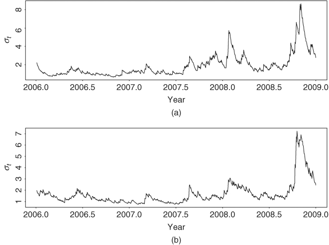
where all of the parameter estimates are significant at the 5% level except for the constant term of the mean equation for the Nikkei 225 index returns. The Ljung–Box statistics of the standardized residuals and their squared series of the two univariate models fail to indicate any model inadequacy. The two volatility equations are close to an IGARCH(1,1) model. This is reasonable because of the increased volatility caused by the subprime financial crisis. Figure 10.2 shows the estimated volatilities of the two univariate GARCH(1,1) models. Indeed, the volatility series confirm that both markets were more volatile than usual in 2008.
Figure 10.1 Time plots of daily log returns in percentages of stock market indexes for Hong Kong and Japan from January 4, 2006, to December 30, 2008: (a) Hong Kong market and (b) Japanese market.
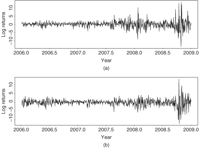
Figure 10.2 Estimated volatilities (standard error) for daily log returns in percentages of stock market indexes for Hong Kong and Japan from January 4, 2006, to December 30, 2008: (a) Hong Kong market and (b) Japanese market. Univariate models are used.
Turn to bivariate modeling. We apply the EWMA approach to obtain volatility estimates, using the command mgarch in S-Plus FinMetrics:
> m3=mgarch(formula.mean=∼arma(0,0),formula.var=∼ewma1,
series=rtn,trace=F)
> summary(m3)
Call:
mgarch(formula.mean =∼arma(0,0), formula.var=∼ewma1,
series=rtn,trace = F)
Mean Equation: structure(.Data = ∼arma(0,0), class="formula")
Conditional Var. Eq.: structure(.Data=∼ewma1,class="formula")
Conditional Distribution: gaussian
--------------------------------------------------------------
Estimated Coefficients:
--------------------------------------------------------------
Value Std.Error t value Pr(>|t|)
C(1) 0.082425 0.030900 2.6675 0.007816
C(2) -0.006849 0.030093 -0.2276 0.820020
ALPHA 0.069492 0.004945 14.0517 0.000000
The estimate of λ is ![]() , which is in the typical range commonly seen in practice. Figure 10.3 shows the estimated volatility series by the EWMA approach. Compared with those in Figure 10.2, the EWMA approach produces smoother volatility series, even though the two plots show similar volatility patterns.
, which is in the typical range commonly seen in practice. Figure 10.3 shows the estimated volatility series by the EWMA approach. Compared with those in Figure 10.2, the EWMA approach produces smoother volatility series, even though the two plots show similar volatility patterns.
Figure 10.3 Estimated volatilities (standard error) for daily log returns in percentages of stock market indices for Hong Kong and Japan from January 4, 2006, to December 30, 2008: (a) Hong Kong market and (b) Japanese market. Exponentially weighted moving-average approach is used.
