
We illustrate the application of multivariate volatility models by considering the value at risk (VaR) of a financial position with multiple assets. Suppose that an investor holds a long position in the stocks of Cisco Systems and Intel Corporation each worth $1 million. We use the daily log returns for the two stocks from January 2, 1991, to December 31, 1999, to build volatility models. The VaR is computed using the 1-step-ahead forecasts at the end of data span and 5% critical values.
Let VaR1 be the value at risk for holding the position on Cisco Systems stock and VaR2 for holding Intel stock. Results of Chapter 7 show that the overall daily VaR for the investor is
![]()
In this illustration, we consider three approaches to volatility modeling for calculating VaR. For simplicity, we do not report standard errors for the parameters involved or model checking statistics. Yet all of the estimates are statistically significant at the 5% level, and the models are adequate based on the Ljung–Box statistics of the standardized residual series and their squared series. The log returns are in percentages so that the quantiles are divided by 100 in VaR calculations. Let r1t be the return of Cisco stock and r2t the return of Intel stock.
Univariate Models
This approach uses a univariate volatility model for each stock return and uses the sample correlation coefficient of the stock returns to estimate ρ. The univariate volatility models for the two stock returns are
![]()
and
![]()
The sample correlation coefficient is 0.473. The 1-step-ahead forecasts needed in VaR calculation at the forecast origin t = 2275 are
![]()
The 5% quantiles for both daily returns are
![]()
where the negative sign denotes loss. For the individual stocks, VaR1 = $1000000q1/100 = $27, 360andVaR2 = $1000000q2/100 = $38, 840. Consequently, the overall VaR for the investor is VaR = $57, 117.
Constant-Correlation Bivariate Model
This approach employs a bivariate GARCH(1,1) model for the stock returns. The correlation coefficient is assumed to be constant over time, but it is estimated jointly with other parameters. The model is

and ![]() . This is a diagonal bivariate GARCH(1,1) model. The 1-step-ahead forecasts for VaR calculation at the forecast origin t = 2275 are
. This is a diagonal bivariate GARCH(1,1) model. The 1-step-ahead forecasts for VaR calculation at the forecast origin t = 2275 are
![]()
Consequently, we have VaR1 = $30, 432 and VaR2 = $37, 195. The overall 5% VaR for the investor is VaR = $58, 180.
Time-Varying Correlation Model
Finally, we allow the correlation coefficient to evolve over time by using the Cholesky decomposition. The fitted model is
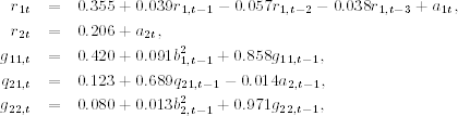
where b1t = a1t and b2t = a2t − q21, ta1t. The 1-step-ahead forecasts for VaR calculation at the forecast origin t = 2275 are
![]()
Therefore, we have ![]() = 4.252,
= 4.252, ![]() , and
, and ![]() . The correlation coefficient is
. The correlation coefficient is ![]() . Using these forecasts, we have VaR1 = $30, 504, VaR2 = $39, 512, and the overall VaR = $57, 648.
. Using these forecasts, we have VaR1 = $30, 504, VaR2 = $39, 512, and the overall VaR = $57, 648.
The estimated VaR values of the three approaches are similar. The univariate models give the lowest VaR, whereas the constant-correlation model produces the highest VaR. The range of the difference is about $1100. The time-varying volatility model seems to produce a compromise between the two extreme models.