
12.5 Linear Regression with Time Series Errors
We are ready to consider some specific applications of MCMC methods. Examples discussed in the next few sections are for illustrative purposes only. The goal here is to highlight the applicability and usefulness of the methods. Understanding these examples can help readers gain insights into applications of MCMC methods in finance.
The first example is to estimate a regression model with serially correlated errors. This is a topic discussed in Chapter 2, where we use SCA to perform the estimation. A simple version of the model is
![]()
where yt is the dependent variable, xit are explanatory variables that may contain lagged values of yt, and zt follows a simple AR(1) model with {at} being a sequence of independent and identically distributed normal random variables with mean zero and variance σ2. Denote the parameters of the model by ![]() , where
, where ![]() , and let
, and let ![]() be the vector of all regressors at time t, including a constant of unity. The model becomes
be the vector of all regressors at time t, including a constant of unity. The model becomes
where n is the sample size.
A natural way to implement Gibbs sampling in this case is to iterate between regression estimation and time series estimation. If the time series model is known, we can estimate the regression model easily by using the least-squares method. However, if the regression model is known, we can obtain the time series zt by using ![]() and use the series to estimate the AR(1) model. Therefore, we need the following conditional posterior distributions:
and use the series to estimate the AR(1) model. Therefore, we need the following conditional posterior distributions:
![]()
where ![]() and X denotes the collection of all observations of explanatory variables.
and X denotes the collection of all observations of explanatory variables.
We use conjugate prior distributions to obtain closed-form expressions for the conditional posterior distributions. The prior distributions are
where again ∼ denotes distribution, and βo, Σo, λ, v, ϕo, and ![]() are known quantities. These quantities are referred to as hyperparameters in Bayesian inference. Their exact values depend on the problem at hand. Typically, we assume that βo = 0, ϕo = 0, and Σo is a diagonal matrix with large diagonal elements. The prior distributions in Eq. (12.7) are assumed to be independent of each other. Thus, we use independent priors based on the partition of the parameter vector θ.
are known quantities. These quantities are referred to as hyperparameters in Bayesian inference. Their exact values depend on the problem at hand. Typically, we assume that βo = 0, ϕo = 0, and Σo is a diagonal matrix with large diagonal elements. The prior distributions in Eq. (12.7) are assumed to be independent of each other. Thus, we use independent priors based on the partition of the parameter vector θ.
The conditional posterior distribution ![]() can be obtained by using Result 12.1a of Section 12.3. Specifically, given ϕ, we define
can be obtained by using Result 12.1a of Section 12.3. Specifically, given ϕ, we define
![]()
Using Eq. (12.6), we have
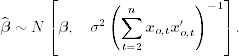
Under the assumption of {at}, Eq. (12.8) is a multiple linear regression. Therefore, information of the data about the parameter vector β is contained in its least-squares estimate
![]()
which has a multivariate normal distribution
Using Result 12.1a, the posterior distribution of β, given the data, ϕ, and σ2, is multivariate normal. We write the result as
where the parameters are given by
![]()
Next, consider the conditional posterior distribution of ϕ given β, σ2, and the data. Because β is given, we can calculate ![]() for all t and consider the AR(1) model
for all t and consider the AR(1) model
![]()
The information of the likelihood function about ϕ is contained in the least-squares estimate
![]()
which is normally distributed with mean ϕ and variance ![]() . Based on Result 12.1, the posterior distribution of ϕ is also normal with mean ϕ* and variance
. Based on Result 12.1, the posterior distribution of ϕ is also normal with mean ϕ* and variance ![]() , where
, where
Finally, turn to the posterior distribution of σ2 given β, ϕ, and the data. Because β and ϕ are known, we can calculate
![]()
By Result 12.8, the posterior distribution of σ2 is an inverted chi-squared distribution—that is,
where ![]() denotes a chi-squared distribution with k degrees of freedom.
denotes a chi-squared distribution with k degrees of freedom.
Using the three conditional posterior distributions in Eqs. (12.9)–(12.11), we can estimate Eq. (12.6) via Gibbs sampling as follows:
1. Specify the hyperparameter values of the priors in Eq. (12.7).
2. Specify arbitrary starting values for β, ϕ, and σ2 (e.g., the ordinary least-squares estimate of β without time series errors).
3. Use the multivariate normal distribution in Eq. (12.9) to draw a random realization for β.
4. Use the univariate normal distribution in Eq. (12.10) to draw a random realization for ϕ.
5. Use the chi-squared distribution in Eq. (12.11) to draw a random realization for σ2.
Repeat steps 3–5 for many iterations to obtain a Gibbs sample. The sample means are then used as point estimates of the parameters of model (12.6).
Example 12.1
As an illustration, we revisit the example of U.S. weekly interest rates of Chapter 2. The data are the 1-year and 3-year Treasury constant maturity rates from January 5, 1962, to April 10, 2009, and are obtained from the Federal Reserve Bank of St. Louis. Because of unit-root nonstationarity, the dependent and independent variables are
1.
c3t = r3t − r3, t−1, which is the weekly change in 3-year maturity rate,
2.
c1t = r1t − r1, t−1, which is the weekly change in 1-year maturity rate,
where the original interest rates rit are measured in percentages. In Chapter 2, we employed a linear regression model with an MA(1) error for the data. Here we consider an AR(2) model for the error process. Using the traditional approach in R, we obtain the model
where ![]() = 0.068. Standard errors of the coefficient estimates of Eq. (12.12) are 0.0075, 0.0201, and 0.0201, respectively. Except for a marginally significant residual ACF at lags 4 and 6, the prior model seems adequate.
= 0.068. Standard errors of the coefficient estimates of Eq. (12.12) are 0.0075, 0.0201, and 0.0201, respectively. Except for a marginally significant residual ACF at lags 4 and 6, the prior model seems adequate.
Writing the model as
where {at} is an independent sequence of N(0, σ2) random variables, we estimate the parameters by Gibbs sampling. The prior distributions used are
![]()
The initial parameter estimates are obtained by the ordinary least-squares method [i.e., by using a two-step procedure of fitting the linear regression model first, then fitting an AR(2) model to the regression residuals]. Since the sample size 2466 is large, the initial estimates are close to those given in Eq. (12.12). We iterated the Gibbs sampling for 2100 iterations but discard results of the first 100 iterations. Table 12.1 gives the posterior means and standard errors of the parameters. From the table, the posterior mean of σ is approximately 0.069. Figure 12.1 shows the time plots of the 2000 Gibbs draws of the parameters. The plots show that the draws are stable. Figure 12.2 gives the histogram of the marginal posterior distribution of each parameter.
Figure 12.1 Time plots of Gibbs draws for the model in Eq. (12.13) with 2100 iterations. Results are based on last 2000 draws. Prior distributions and starting parameter values are given in text.

Figure 12.2 Histograms of Gibbs draws for model in Eq. (12.13) with 2100 iterations. Results are based on last 2000 draws. Prior distributions and starting parameter values are given in text.

Table 12.1 Posterior Means and Standard Errors of Model (12.13) Estimated by Gibbs Sampling with 2100 Iterationsa

a
The results are based on the last 2000 iterations, and the prior distributions are given in the text.
We repeated the Gibbs sampling with different initial values but obtained similar results. The Gibbs sampling appears to have converged. From Table 12.1, the posterior means are close to the estimates of Eq. (12.12).This is expected as the sample size is large and the model is relatively simple.