The Markov switching model is another econometric model for which MCMC methods enjoy many advantages over the traditional likelihood method. McCulloch and Tsay (1994b) discuss a Gibbs sampling procedure to estimate such a model when the volatility in each state is constant over time. These authors applied the procedure to estimate a Markov switching model with different dynamics and mean levels for different states to the quarterly growth rate of U.S. real gross national product, seasonally adjusted, and obtained some interesting results. For instance, the dynamics of the growth rate are significantly different between periods of economic “contraction” and “expansion.” Since this chapter is concerned with asset returns, we focus on models with volatility switching.
Suppose that an asset return rt follows a simple two-state Markov switching model with different risk premiums and different GARCH dynamics:

where ![]() , {ϵt} is a sequence of Gaussian white noises with mean zero and variance 1, and the parameters αij satisfy some regularity conditions so that the unconditional variance of at exists. The probability transition from one state to another is governed by
, {ϵt} is a sequence of Gaussian white noises with mean zero and variance 1, and the parameters αij satisfy some regularity conditions so that the unconditional variance of at exists. The probability transition from one state to another is governed by
where 0 < ei < 1. A small ei means that the return series has a tendency to stay in the ith state with expected duration 1/ei. For the model in Eq. (12.55) to be identifiable, we assume that β2 > β1 so that state 2 is associated with higher risk premium. This is not a critical restriction because it is used to achieve uniqueness in labeling the states. A special case of the model results if α1j = α2j for all j so that the model assumes a GARCH model for all states. However, if ![]() is replaced by βi, then model (12.55) reduces to a simple Markov switching GARCH model.
is replaced by βi, then model (12.55) reduces to a simple Markov switching GARCH model.
Model (12.55) is a Markov switching GARCH-M model. For simplicity, we assume that the initial volatility h1 is given with value equal to the sample variance of rt. A more sophisticated analysis is to treat h1 as a parameter and estimate it jointly with other parameters. We expect the effect of fixing h1 will be negligible in most applications, especially when the sample size is large. The “traditional” parameters of the Markov switching GARCH-M model are ![]() ,
, ![]() for i = 1 and 2, and the transition probabilities
for i = 1 and 2, and the transition probabilities ![]() . The state vector
. The state vector ![]() contains the augmented parameters. The volatility vector
contains the augmented parameters. The volatility vector ![]() can be computed recursively if h1,
can be computed recursively if h1, ![]() , and the state vector
, and the state vector ![]() are given.
are given.
Dependence of the return on volatility in model (12.55) implies that the return is also serially correlated. The model thus has some predictability in the return. However, states of the future returns are unknown and a prediction produced by the model is necessarily a mixture of those over possible state configurations. This often results in high uncertainty in point prediction of future returns.
Turn to estimation. The likelihood function of model (12.55) is complicated as it is a mixture over all possible state configurations. Yet the Gibbs sampling approach only requires the following conditional posterior distributions:
![]()
where ![]() is the collection of observed returns. For simplicity, we use conjugate prior distributions discussed in Section 12.3—that is,
is the collection of observed returns. For simplicity, we use conjugate prior distributions discussed in Section 12.3—that is,
![]()
The prior distribution of parameter αij is uniform over a properly specified interval. Since αij is a nonlinear parameter of the likelihood function, we use the Griddy Gibbs to draw its random realizations. A uniform prior distribution simplifies the computation involved. Details of the prior conditional posterior distributions follow:
1. The posterior distribution of βi only depends on the data in state i. Define
![]()
Then we have
![]()
Therefore, information of the data on βi is contained in the sample mean of rit. Let ![]() i =
i = ![]() , where the summation is over all data points in state i and ni is the number of data points in state i. Then the conditional posterior distribution of βi is normal with mean
, where the summation is over all data points in state i and ni is the number of data points in state i. Then the conditional posterior distribution of βi is normal with mean ![]() and variance
and variance ![]() , where
, where
![]()
2. Next, the parameters αij can be drawn one by one using the Griddy Gibbs method. Given h1, ![]() ,
, ![]() , and αiv with v ≠ j, the conditional posterior distribution function of αij does not correspond to a well-known distribution, but it can be evaluated easily as
, and αiv with v ≠ j, the conditional posterior distribution function of αij does not correspond to a well-known distribution, but it can be evaluated easily as
![]()
where ht contains αij. We evaluate this function at a grid of points for αij over a properly specified interval. For example, 0 ≤ α11 < 1 − α12.
3. The conditional posterior distribution of ei only involves ![]() . Let ℓ1 be the number of switches from state 1 to state 2 and ℓ2 be the number of switches from state 2 to state 1 in
. Let ℓ1 be the number of switches from state 1 to state 2 and ℓ2 be the number of switches from state 2 to state 1 in ![]() . Also, let ni be the number of data points in state i. Then by Result 12.3 of conjugate prior distributions, the posterior distribution of ei is β(γi1 + ℓi, γi2 + ni − ℓi).
. Also, let ni be the number of data points in state i. Then by Result 12.3 of conjugate prior distributions, the posterior distribution of ei is β(γi1 + ℓi, γi2 + ni − ℓi).
4. Finally, elements of ![]() can be drawn one by one. Let
can be drawn one by one. Let ![]() be the vector obtained by removing sj from
be the vector obtained by removing sj from ![]() . Given
. Given ![]() and other information, sj can assume two possibilities (i.e., sj = 1 or sj = 2), and its conditional posterior distribution is
and other information, sj can assume two possibilities (i.e., sj = 1 or sj = 2), and its conditional posterior distribution is
![]()
The probability
![]()
can be computed by the Markov transition probabilities in Eq. (12.56). In addition, assuming sj = i, one can compute ht for t ≥ j recursively. The relevant likelihood function, denoted by L(sj), is given by
![]()
for i = 1 and 2, where ![]() if st = 1 and
if st = 1 and ![]() otherwise. Consequently, the conditional posterior probability of sj = 1 is
otherwise. Consequently, the conditional posterior probability of sj = 1 is
![]()
The state sj can then be drawn easily using a uniform distribution on the unit interval [0, 1].
Remark
Since sj and sj+1 are highly correlated when e1 and e2 are small, it is more efficient to draw several sj jointly. However, the computation involved in enumerating the possible state configurations increases quickly with the number of states drawn jointly. □
Example 12.6
In this example, we consider the monthly log stock returns of General Electric Company from January 1926 to December 1999 for 888 observations. The returns are in percentages and shown in Figure 12.14(a). For comparison purposes, we start with a GARCH-M model for the series and obtain
where rt is the monthly log return and {ϵt} is a sequence of independent Gaussian white noises with mean zero and variance 1. All parameter estimates are highly significant with p values less than 0.0006. The Ljung–Box statistics of the standardized residuals and their squared series fail to suggest any model inadequacy. It is reassuring to see that the risk premium is positive and significant. The GARCH model in Eq. (12.57) can be written as
![]()
where ![]() and B is the back-shift operator such that
and B is the back-shift operator such that ![]() =
= ![]() . As discussed in Chapter 3, the prior equation can be regarded as an ARMA(2,1) model with nonhomogeneous innovations for the squared series
. As discussed in Chapter 3, the prior equation can be regarded as an ARMA(2,1) model with nonhomogeneous innovations for the squared series ![]() . The AR polynomial can be factorized as (1 − 0.945B)(1 − 0.820B), indicating two real characteristic roots with magnitudes less than 1. Consequently, the unconditional variance of rt is finite and equal to 0.546/(1 − 1.765 + 0.775) ≈ 49.64.
. The AR polynomial can be factorized as (1 − 0.945B)(1 − 0.820B), indicating two real characteristic roots with magnitudes less than 1. Consequently, the unconditional variance of rt is finite and equal to 0.546/(1 − 1.765 + 0.775) ≈ 49.64.
Figure 12.14 (a) Time plot of monthly log returns, in percentages, of GE stock from 1926 to 1999. (b) Time plot of the posterior probability of being in state 2 based on results of last 2000 iterations of Gibbs sampling with 5000 + 2000 total iterations. Model used is two-state Markov switching GARCH-M model.

Turn to Markov switching models. We use the following prior distributions:
![]()
The initial parameter values used are (a) ei = 0.1, (b) s1 is a Bernoulli trial with equal probabilities and st is generated sequentially using the initial transition probabilities, and (c) ![]() and
and ![]() . Gibbs samples of αij are drawn using the Griddy Gibbs with 400 grid points, equally spaced over the following ranges: αi0 ε [0, 6.0], αi1 ε [0, 1], and αi2 ε [0, 0.5]. In addition, we implement the constraints αi1 + αi2 < 1 for i = 1, 2. The Gibbs sampler is run for 5000 + 2000 iterations, but only results of the last 2000 iterations are used to make inference.
. Gibbs samples of αij are drawn using the Griddy Gibbs with 400 grid points, equally spaced over the following ranges: αi0 ε [0, 6.0], αi1 ε [0, 1], and αi2 ε [0, 0.5]. In addition, we implement the constraints αi1 + αi2 < 1 for i = 1, 2. The Gibbs sampler is run for 5000 + 2000 iterations, but only results of the last 2000 iterations are used to make inference.
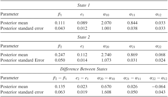
Table 12.5 shows the posterior means and standard deviations of parameters of the Markov switching GARCH-M model in Eq. (12.55). In particular, it also contains some statistics showing the difference between the two states such as θ = β2 − β1. The difference between the risk premiums is statistically significant at the 5% level. The differences in posterior means of the volatility parameters between the two states appear to be insignificant. Yet the posterior distributions of volatility parameters show some different characteristics. Figures 12.15 and 12.16 show the histograms of all parameters in the Markov switching GARCH-M model. They exhibit some differences between the two states. Figure 12.17 shows the time plot of the persistent parameter αi1 + αi2 for the two states. It shows that the persistent parameter of state 1 reaches the boundary 1.0 frequently, but that of state 2 does not. The expected durations of the two states are about 11 and 9 months, respectively. Figure 12.14(b) shows the posterior probability of being in state 2 for each observation.
Figure 12.15 Histograms of risk premium and transition probabilities of a two-state Markov switching GARCH-M model for monthly log returns of GE stock from 1926 to 1999. Results based on last 2000 iterations of Gibbs sampling with 5000 + 2000 total iterations.
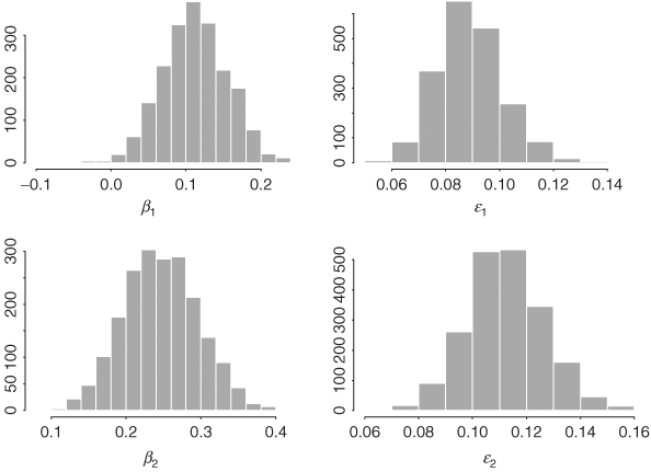
Figure 12.16 Histograms of volatility parameters of two-state Markov switching GARCH-M model for monthly log returns of GE stock from 1926 to 1999. Results based on last 2000 iterations of Gibbs sampling with 5000 + 2000 total iterations.
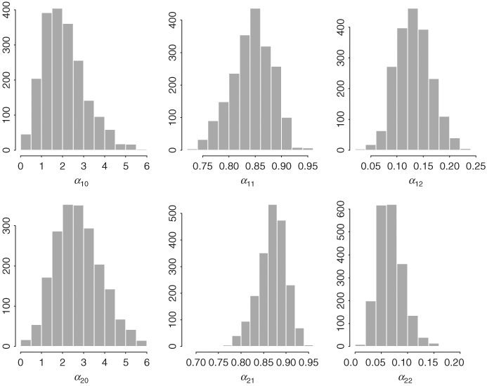
Figure 12.17 Time plots of persistent parameter αi1 + αi2 of two-state Markov switching GARCH-M model for monthly log returns of GE stock from 1926 to 1999. Results based on last 2000 iterations of Gibbs sampling with 5000 + 2000 total iterations.

Table 12.5 Fitted Markov Switching GARCH-M Model for Monthly Log Returns of GE Stock from January 1926 to December 1999a
a
The numbers shown are the posterior means and standard deviations based on a Gibbs sampling with 5000 + 2000 iterations. Results of the first 5000 iterations are discarded. The prior distributions and initial parameter estimates are given in the text.
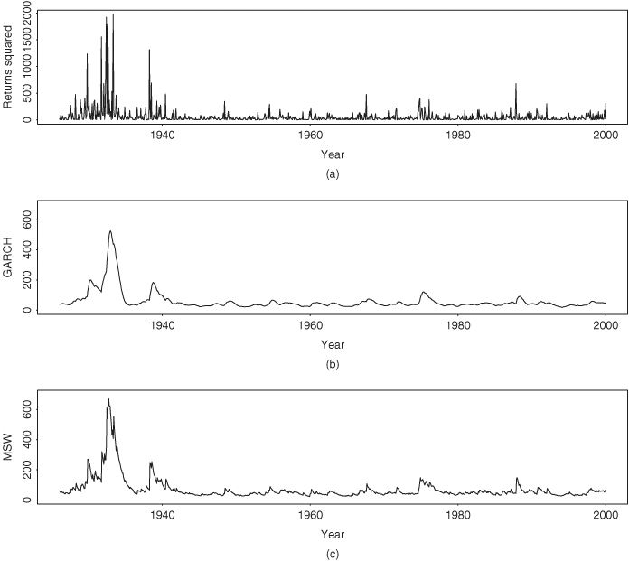
Finally, we compare the fitted volatility series of the simple GARCH-M model in Eq. (12.57) and the Markov switching GARCH-M model in Eq. (12.55). The two fitted volatility series (Figure 12.18) show similar patterns and are consistent with the behavior of the squared log returns. The simple GARCH-M model produces a smoother volatility series with lower estimated volatilities.
Figure 12.18 Fitted volatility series for monthly log returns of GE stock from 1926 to 1999: (a) squared log returns, (b) GARCH-M model in Eq. (12.59), and (c) two-state Markov switching GARCH-M model in Eq. (12.57).