
Unlike the linear model, there exist no closed-form formulas to compute forecasts of most nonlinear models when the forecast horizon is greater than 1. We use parametric bootstraps to compute nonlinear forecasts. It is understood that the model used in forecasting has been rigorously checked and is judged to be adequate for the series under study. By a model, we mean the dynamic structure and innovational distributions. In some cases, we may treat the estimated parameters as given.
4.4.1 Parametric Bootstrap
Let T be the forecast origin and ℓ be the forecast horizon (ℓ > 0). That is, we are at time index T and interested in forecasting xT+ℓ. The parametric bootstrap considered computes realizations xT+1, … , XT+ℓ sequentially by (a) drawing a new innovation from the specified innovational distribution of the model, and (b) computing xT+i using the model, data, and previous forecasts xT+1, … , xT+i−1. This results in a realization for xT+ℓ. The procedure is repeated M times to obtain M realizations of xT+ℓ denoted by ![]() . The point forecast of xT+ℓ is then the sample average of
. The point forecast of xT+ℓ is then the sample average of ![]() . Let the forecast be xT(ℓ). We used M = 3000 in some applications and the results seem fine. The realizations
. Let the forecast be xT(ℓ). We used M = 3000 in some applications and the results seem fine. The realizations ![]() can also be used to obtain an empirical distribution of xT+ℓ. We make use of this empirical distribution later to evaluate forecasting performance.
can also be used to obtain an empirical distribution of xT+ℓ. We make use of this empirical distribution later to evaluate forecasting performance.
4.4.2 Forecasting Evaluation
There are many ways to evaluate the forecasting performance of a model, ranging from directional measures to magnitude measures to distributional measures. A directional measure considers the future direction (up or down) implied by the model. Predicting that tomorrow's S&P 500 index will go up or down is an example of directional forecasts that are of practical interest. Predicting the year-end value of the daily S&P 500 index belongs to the case of magnitude measure. Finally, assessing the likelihood that the daily S&P 500 index will go up 10% or more between now and the year end requires knowing the future conditional probability distribution of the index. Evaluating the accuracy of such an assessment needs a distributional measure.
In practice, the available data set is divided into two subsamples. The first subsample of the data is used to build a nonlinear model, and the second subsample is used to evaluate the forecasting performance of the model. We refer to the two subsamples of data as estimation and forecasting subsamples. In some studies, a rolling forecasting procedure is used in which a new data point is moved from the forecasting subsample into the estimation subsample as the forecast origin advances. In what follows, we briefly discuss some measures of forecasting performance that are commonly used in the literature. Keep in mind, however, that there exists no widely accepted single measure to compare models. A utility function based on the objective of the forecast might be needed to better understand the comparison.
Directional Measure
A typical measure here is to use a 2 × 2 contingency table that summarizes the number of “hits” and “misses” of the model in predicting ups and downs of xT+ℓ in the forecasting subsample. Specifically, the contingency table is given as

where m is the total number of ℓ-step-ahead forecasts in the forecasting subsample, m11 is the number of “hits” in predicting upward movements, m21 is the number of “misses” in predicting downward movements of the market, and so on. Larger values in m11 and m22 indicate better forecasts. The test statistic
![]()
can then be used to evaluate the performance of the model. A large χ2 signifies that the model outperforms the chance of random choice. Under some mild conditions, χ2 has an asymptotic chi-squared distribution with 1 degree of freedom. For further discussion of this measure, see Dahl and Hylleberg (1999).
For illustration of the directional measure, consider the 1-step-ahead probability forecasts of the 8–4–1 feed-forward neural network shown in Figure 4.9. The 2 × 2 table of “hits” and “misses” of the network is
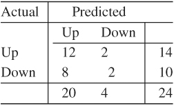
The table shows that the network predicts the upward movement well, but fares poorly in forecasting the downward movement of the stock. The chi-squared statistic of the table is 0.137 with a p value of 0.71. Consequently, the network does not significantly outperform a random-walk model with equal probabilities for “upward” and “downward” movements.
Magnitude Measure
Three statistics are commonly used to measure performance of point forecasts. They are the mean squared error (MSE), mean absolute deviation (MAD), and mean absolute percentage error (MAPE). For ℓ-step-ahead forecasts, these measures are defined as
4.49 ![]()
4.50 ![]()
4.51 ![]()
where m is the number of ℓ-step-ahead forecasts available in the forecasting subsample. In application, one often chooses one of the above three measures, and the model with the smallest magnitude on that measure is regarded as the best ℓ-step-ahead forecasting model. It is possible that different ℓ may result in selecting different models. The measures also have other limitations in model comparison; see, for instance, Clements and Hendry (1993).
Distributional Measure
Practitioners recently began to assess forecasting performance of a model using its predictive distributions. Strictly speaking, a predictive distribution incorporates parameter uncertainty in forecasts. We call it conditional predictive distribution if the parameters are treated as fixed. The empirical distribution of xT+ℓ obtained by the parametric bootstrap is a conditional predictive distribution. This empirical distribution is often used to compute a distributional measure. Let uT(ℓ) be the percentile of the observed xT+ℓ in the prior empirical distribution. We then have a set of m percentiles ![]() , where again m is the number of ℓ-step-ahead forecasts in the forecasting subsample. If the model entertained is adequate, {uT+j(ℓ)} should be a random sample from the uniform distribution on [0, 1]. For a sufficiently large m, one can compute the Kolmogorov–Smirnov statistic of {uT+j(ℓ)} with respect to uniform [0, 1]. The statistic can be used for both model checking and forecasting comparison.
, where again m is the number of ℓ-step-ahead forecasts in the forecasting subsample. If the model entertained is adequate, {uT+j(ℓ)} should be a random sample from the uniform distribution on [0, 1]. For a sufficiently large m, one can compute the Kolmogorov–Smirnov statistic of {uT+j(ℓ)} with respect to uniform [0, 1]. The statistic can be used for both model checking and forecasting comparison.