
In this section we apply the ACD model to stock volatility modeling. Consider the daily range of the log price of Apple stock from January 4, 1999, to November 20, 2007. The data are obtained from Yahoo Finance and consist of 2235 observations. This series was analyzed in Tsay (2009). The range of daily log prices has been used in the literature as a robust alternative to volatility modeling; see Chapter 3 and Chou (2005) and the references therein. Apple stock had two-for-one splits on June 21, 2000, and February 28, 2005, during the sample period, but no adjustments are needed for the splits because we use daily range of log price. As mentioned before, stock prices in the U.S. markets switched from the tick size ![]() of a dollar to the decimal system on January 29, 2001. Such a change affected the bid–ask spread of stock prices. We shall employ intervention analysis to study the impact of such a policy change on the stock volatility.
of a dollar to the decimal system on January 29, 2001. Such a change affected the bid–ask spread of stock prices. We shall employ intervention analysis to study the impact of such a policy change on the stock volatility.
The sample mean, standard deviation, minimum, and maximum of the range of log prices are 0.0407, 0.0218, 0.0068, and 0.1468, respectively. The sample skewness and excess kurtosis are 1.3 and 2.13, respectively. Figure 5.18(a) shows the time plot of the range series. The volatility seems to be increasing from 2000 to 2001, then decreasing to a stable level after 2002. It seems to increase somewhat at the end of the series. Figure 5.19(a) shows the sample ACF of the daily range series. The sample ACFs are highly significant and decay slowly.
Figure 5.18 Time plots of daily range of log price of Apple stock from January 4, 1999, to November 20, 2007: (a) observed daily range and (b) standardized residuals of a GACD(1,1) model.
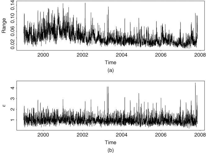
Figure 5.19 Sample autocorrelation function of daily range of log prices of Apple stock from January 4, 1999, to November 20, 2007: (a) ACF of daily range and (b) ACF of standardized residual series of GACD(1,1) model.

We fit EACD(1,1), WACD(1,1), and GACD(1,1) models to the daily range series. The estimation results, along with the Ljung–Box statistics for the standardized residual series and its squared process, are given in Table 5.9. The parameter estimates for the duration equation are stable for all three models, except for the constant term of the EACD model, which appears to be statistically insignificant at the usual 5% level. Indeed, in this particular instance, the EACD(1,1) model fares slightly worse than the other two ACD models. Between the WACD(1,1) and GACD(1,1) models, we slightly prefer the GACD(1,1) model because it fits the data better and is more flexible.
Table 5.9 Estimation Results of EACD(1,1), WACD(1,1), and GACD(1,1) Models for Daily Range of Log Prices of Apple Stock from January 4, 1999 to November 20, 2007a

aThe standard errors of the estimates and the p values of the Ljung–Box statistics are in parentheses, where Q(10) and Q*(10) are for standardized residual series and its squared process, respectively.
Figure 5.19(b) shows the sample ACFs of the standardized residuals of the fitted GACD(1,1) model. From the plot, the standardized residuals do not have significant serial correlations, even though the lag-1 sample ACF is slightly above its two standard error limit. The lag-1 serial correlation is removed when we use nonlinear ACD models later. Figure 5.18(b) shows the time plot of the standardized residuals of the GACD(1,1) model. The residuals do not show any pattern of model inadequacy. The mean, standard deviation, minimum, and maximum of the standardized residuals are 0.203, 4.497, 0.999, and 0.436, respectively.
It is interesting to see that the estimates of the shape parameter α are greater than 1 for both WACD(1,1) and GACD(1,1) models, indicating that the hazard function of the daily range is monotonously increasing. This is consistent with the idea of volatility clustering, for large volatility tends to be followed by another large volatility.
Threshold ACD model
To refine the GACD(1,1) model for the daily range of log prices of Apple stock, we employ a two-regime threshold WACD(1,1) model. Some preliminary analysis of the threshold WACD models indicates that the major difference in the parameter estimates between the two regimes is the shape parameter of the Weibull distribution. Thus, we focus on a TWACD(2;1,1) model with different shape parameters for the two regimes.
Table 5.10 gives the maximized log-likelihood value of a TWACD(2;1,1) model with delay d = 1 and threshold r ∈ {x(q)|q = 60, 65, … , 95}, where x(q) denotes the sample qth percentile. From the table, the threshold 0.04753 is selected, which is the 70th percentile of the data. The fitted model is
![]()
where the standard errors of the coefficients are 0.0003, 0.0164, and 0.0215, respectively, and ϵi follows the standardized Weibull distribution as
![]()
where the standard errors of the two shape parameters are 0.0394 and 0.0717, respectively.
Table 5.10 Selection of Threshold of TWACD(2;1,1) Model for Daily Range of Log Prices of Apple Stock from January 4, 1999, to November 20, 2007a
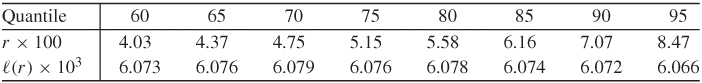
aThe threshold variable is xi−1.
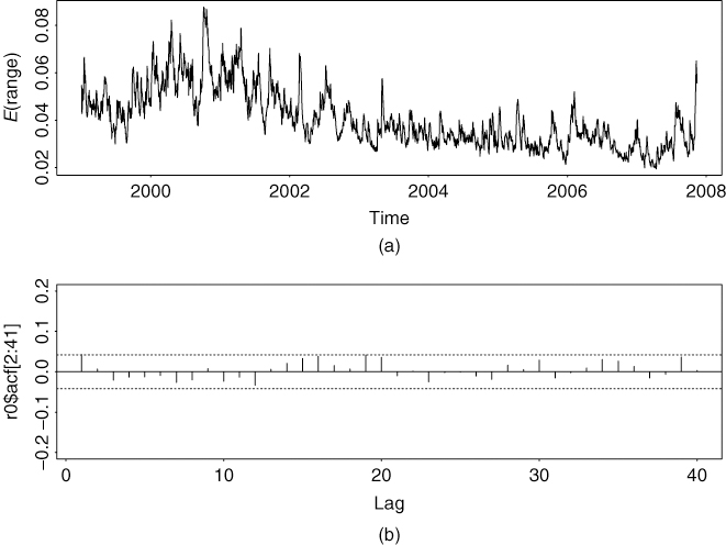
Figure 5.20(a) shows the time plot of the conditional expected duration for the fitted TWACD(2;1,1) model, that is, ![]() , whereas Figure 5.20(b) gives the residual ACFs for the fitted model. All residual ACFs are within the two standard error limits. Indeed, we have Q(1) = 4.01(0.05) and Q(10) = 9.84(0.45) for the standardized residuals and Q*(1) = 0.83(0.36) and Q*(10) = 9.35(0.50) for the squared series of the standardized residuals, where the number in parentheses denotes p value. Note that the threshold variable xi−1 is also selected based on the value of the log-likelihood function. For instance, the log-likelihood function of the TWACD(2;1,1) model assumes the value 6.069 × 10³ and 6.070 × 10³, respectively, for d = 2 and 3 when the threshold is 0.04753. These values are lower than that when d = 1.
, whereas Figure 5.20(b) gives the residual ACFs for the fitted model. All residual ACFs are within the two standard error limits. Indeed, we have Q(1) = 4.01(0.05) and Q(10) = 9.84(0.45) for the standardized residuals and Q*(1) = 0.83(0.36) and Q*(10) = 9.35(0.50) for the squared series of the standardized residuals, where the number in parentheses denotes p value. Note that the threshold variable xi−1 is also selected based on the value of the log-likelihood function. For instance, the log-likelihood function of the TWACD(2;1,1) model assumes the value 6.069 × 10³ and 6.070 × 10³, respectively, for d = 2 and 3 when the threshold is 0.04753. These values are lower than that when d = 1.
Figure 5.20 Model fitting for daily range of log price of Apple stock from January 4, 1999, to November 20, 2007: (a) conditional expected durations of fitted TWACD(2;1,1) model and (b) sample ACF of standardized residuals.
Intervention Analysis
High-frequency financial data are often influenced by external events, for example, an increase or drop in interest rates by the U.S. Federal Open Market Committee or a jump in the oil price. Applications of ACD models in finance are often faced with the problem of outside interventions. To handle the effects of external events, the intervention analysis of Box and Tiao (1975) can be used. Here we apply the analysis to the daily range series of Apple stock to study the impact of change in tick size on the stock volatility.
Let to be the time of intervention. For the Apple stock, to = 522, which corresponds to January 26, 2001, the last trading day before the change in tick size. Since more observations in the sample are after the intervention, we define the indicator variable
![]()
to signify the absence of intervention. Since a larger tick size tends to increase the observed daily price range, it is reasonable to assume that the conditional expected range would be higher before the intervention. A simple intervention model for the daily range of Apple stock is then given by
![]()
where ψi follows the model
5.54 ![]()
where γ denotes the decrease in expected duration due to the decimalization of stock prices. In other words, the expected durations before and after the intervention are
![]()
respectively. We expect γ > 0.
The fitted duration equation for the intervention model is
![]()
where the standard errors of the estimates are 0.0004, 0.0003, 0.0177, and 0.0264, respectively. The estimate ![]() is significant at the 1% level. For the innovations, we have
is significant at the 1% level. For the innovations, we have
![]()
The standard errors of the two estimates of the shape parameter are 0.0413 and 0.0780, respectively. Figure 5.21(a) shows the expected durations of the intervention model, and Figure 5.21(b) shows the ACF of the standardized residuals. All residual ACFs are within the two standard error limits. Indeed, for the standardized residuals, we have Q(1) = 2.37(0.12) and Q(10) = 6.24(0.79). For the squared series of the standardized residuals, we have Q*(1) = 0.34(0.56) and Q*(10) = 6.79(0.75). As expected, ![]() so that the decimalization indeed reduces the expected value of the daily range. This simple analysis shows that, as expected, adopting the decimal system reduces the volatility of Apple stock.
so that the decimalization indeed reduces the expected value of the daily range. This simple analysis shows that, as expected, adopting the decimal system reduces the volatility of Apple stock.
Figure 5.21 Model fitting for daily range of log price of Apple stock from January 4, 1999, to November 20, 2007: (a) conditional expected durations of fitted TWACD(2;1,1) model with intervention and (b) sample ACF of corresponding standardized residuals.
