
6.6 Black–Scholes Pricing Formulas
Black and Scholes (1973) successfully solved their differential equation in Eq. (6.17) to obtain exact formulas for the price of European call-and-put options. In what follows, we derive these formulas using what is called risk-neutral valuation in finance.
6.6.1 Risk-Neutral World
The drift parameter μ drops out from the Black–Scholes differential equation. In finance, this means the equation is independent of risk preferences. In other words, risk preferences cannot affect the solution of the equation. A nice consequence of this property is that one can assume that investors are risk neutral. In a risk-neutral world, we have the following results:
- The expected return on all securities is the risk-free interest rate r.
- The present value of any cash flow can be obtained by discounting its expected value at the risk-free rate.
6.6.2 Formulas
The expected value of a European call option at maturity in a risk-neutral world is
![]()
where E* denotes expected value in a risk-neutral world. The price of the call option at time t is
Yet in a risk-neutral world, we have μ = r, and by Eq. (6.10), ln(PT) is normally distributed as
![]()
Let g(PT) be the probability density function of PT. Then the price of the call option in Eq. (6.18) is
![]()
By changing the variable in the integration and some algebraic calculations (details are given in Appendix A), we have
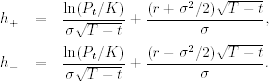
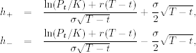
where Φ(x) is the cumulative distribution function (CDF) of the standard normal random variable evaluated at x,

In practice, Φ(x) can easily be obtained from most statistical packages. Alternatively, one can use an approximation given in Appendix B.
The Black–Scholes call formula in Eq. (6.19) has some nice interpretations. First, if we exercise the call option on the expiration date, we receive the stock, but we have to pay the strike price. This exchange will take place only when the call finishes in-the-money (i.e., PT > K). The first term PtΦ(h+) is the present value of receiving the stock if and only if PT > K and the second term − K exp[ − r(T − t)]Φ(h−) is the present value of paying the strike price if and only if PT > K. A second interpretation is particularly useful. As shown in the derivation of the Black–Scholes differential equation in Section 6.5, Φ(h+) = ∂Gt/∂Pt is the number of shares in the portfolio that does not involve uncertainty, the Wiener process. This quantity is known as the delta in hedging. We know that ct = PtΦ(h+) + Bt, where Bt is the dollar amount invested in risk-free bonds in the portfolio (or short on the derivative). We can then see that Bt = − K exp[ − r(T − t)]Φ(h−) directly from inspection of the Black–Scholes formula. The first term of the formula, PtΦ(h+), is the amount invested in the stock, whereas the second term, K exp[ − r(T − t)]Φ(h−), is the amount borrowed.
Similarly, we can obtain the price of a European put option as
(6.20) ![]()
Since the standard normal distribution is symmetric with respect to its mean 0.0, we have Φ(x) = 1 − Φ( − x) for all x. Using this property, we have Φ( − hi) = 1 − Φ(hi). Thus, the information needed to compute the price of a put option is the same as that of a call option. Alternatively, using the symmetry of normal distribution, it is easy to verify that
![]()
which is referred to as the put–call parity and can be used to obtain pt from ct. The put–call parity can also be obtained by considering the following two portfolios:
1. Portfolio A One European call option plus an amount of cash equal to K exp[ − r(T − t)].
2. Portfolio B One European put option plus one share of the underlying stock.
The payoff of these two portfolios is
![]()
at the expiration of the options. Since the options can only be exercised at the expiration date, the portfolios must have identical value today. This means
![]()
which is the put–call parity given earlier.
Example 6.5
Suppose that the current price of Intel stock is $80 per share with volatility σ = 20% per annum. Suppose further that the risk-free interest rate is 8% per annum. What is the price of a European call option on Intel with a strike price of $90 that will expire in 3 months?
From the assumptions, we have Pt = 80, K = 90, T − t = 0.25, σ = 0.2, and r = 0.08. Therefore,
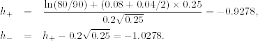
Using any statistical software (e.g., R or S-Plus) or the approximation in Appendix B, we have
![]()
Consequently, the price of a European call option is
![]()
The stock price has to rise by $10.73 for the purchaser of the call option to break even.
Under the same assumptions, the price of a European put option is
![]()
Thus, the stock price can rise an additional $1.05 for the purchaser of the put option to break even.
Example 6.6
The strike price of the previous example is well beyond the current stock price. A more realistic strike price is $81. Assume that the other conditions of the previous example continue to hold. We now have Pt = 80, K = 81, r = 0.08, and T − t = 0.25, and the hi become
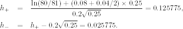
Using the approximation in Appendix B, we have Φ(0.125775) = 0.5500 and Φ(0.025775) = 0.5103. The price of a European call option is then
![]()
The price of the stock has to rise by $4.49 for the purchaser of the call option to break even. On the other hand, under the same assumptions, the price of a European put option is
![]()
The stock price must fall $1.89 for the purchaser of the put option to break even.
6.6.3 Lower Bounds of European Options
Consider the call option of a nondividend-paying stock. It can be shown that the price of a European call option satisfies
![]()
that is, the lower bound for a European call price is Pt − K exp[ − r(T − t)]. This result can be verified by considering two portfolios:
1. Portfolio A. One European call option plus an amount of cash equal to K exp[ − r(T − t)].
2. Portfolio B. One share of the stock.
For portfolio A, if the cash is invested at the risk-free interest rate, it will result in K at time T. If PT > K, the call option is exercised at time T and the portfolio is worth PT. If PT < K, the call option expires worthless and the portfolio is worth K. Therefore, the value of portfolio is
![]()
The value of portfolio B is PT at time T. Hence, portfolio A is always worth more than (or, at least, equal to) portfolio B. It follows that portfolio A must be worth more than portfolio B today; that is,
![]()
Furthermore, since ct ≥ 0, we have
![]()
A similar approach can be used to show that the price of a corresponding European put option satisfies
![]()
Example 6.7
Suppose that Pt = $30, K = $28, r = 6% per annum, and T − t = 0.5. In this case,
![]()
Assume that the European call price of the stock is $2.50, which is less than the theoretical minimum of $2.83. An arbitrageur can buy the call option and short the stock. This provides a new cash flow of $(30 − 2.50) = $27.50. If invested for 6 months at the risk-free interest rate, the $27.50 grows to $27.50 exp(0.06 × 0.5) = $28.34. At the expiration time, if PT > $28, the arbitrageur exercises the option, closes out the short position, and makes a profit of $(28.34 − 28) = $0.34. On the other hand, if PT < $28, the stock is bought in the market to close the short position. The arbitrageur then makes an even greater profit. For illustration, suppose that PT = $27.00, then the profit is $(28.34 − 27.00) = $1.34.
6.6.4 Discussion
From the formulas, the price of a call or put option depends on five variables—namely, the current stock price Pt, the strike price K, the time to expiration T − t measured in years, the volatility σ per annum, and the interest rate r per annum. It pays to study the effects of these five variables on the price of an option.
Marginal Effects
Consider first the marginal effects of the five variables on the price of a call option ct. By marginal effects we mean changing one variable while holding the others fixed. The effects on a call option can be summarized as follows:
1. Current Stock Price Pt ct is positively related to ln(Pt). In particular, ct → 0 as Pt → 0 and ct → ∞ as Pt → ∞. Figure 6.3(a) illustrates the effects with K = 80, r = 6% per annum, T − t = 0.25 year, and σ = 30% per annum.
2. Strike Price K ct is negatively related to ln(K). In particular, ct → Pt as K → 0 and ct → 0 as K → ∞.
3. Time to Expiration ct is related to T − t in a complicated manner, but we can obtain the limiting results by writing h+ and h− as
If Pt < K, then ct → 0 as (T − t) → 0. If Pt > K, then ct → Pt − K as (T − t) → 0 and ct → Pt as (T − t) → ∞. Figure 6.4(a) shows the marginal effects of T − t on ct for three different current stock prices. The fixed variables are K = 80, r = 6%, and σ = 30%. The solid, dotted, and dashed lines of the plot are for Pt = 70, 80, and 90, respectively.
4. Volatility σ Rewriting h+ and h− as
we obtain that (a) if ln(Pt/K) + r(T − t) < 0, then ct → 0 as σ → 0, and (b) if ln(Pt/K) + r(T − t) ≥ 0, then ct → Pt − Ke−r(T−t) as σ → 0 and ct → Pt as σ → ∞. Figure 6.5(a) shows the effects of σ on ct for K = 80, T − t = 0.25, r = 0.06, and three different values of Pt. The solid, dotted, and dashed lines are for Pt = 70, 80, and 90, respectively.
5. Interest Rate ct is positively related to r such that ct → Pt as r → ∞.
Figure 6.3 Marginal effects of current stock price on price of an option with K = 80, T − t = 0.25, σ = 0.3, and r = 0.06: (a) call option and (b) put option.

Figure 6.4 Marginal effects of time to expiration on price of an option with K = 80, σ = 0.3, and r = 0.06: (a) call option and (b) put option. Solid, dotted, and dashed lines are for current stock price Pt = 70, 80, and 90, respectively.
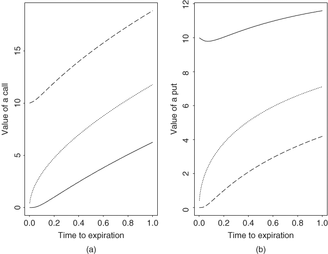
Figure 6.5 Marginal effects of stock volatility on price of an option with K = 80, T − t = 0.25, and r = 0.06: (a) call option and (b) put option. Solid, dotted, and dashed lines are for current stock price Pt = 70, 80, and 90, respectively.

The marginal effects of the five variables on a put option can be obtained similarly. Figures 6.3(b), 6.4(b), and 6.5(b) illustrates the effects for some selected cases.
Some Joint Effects
Figure 6.6 shows the joint effects of volatility and strike price on a call option, where the other variables are fixed at Pt = 80, r = 0.06, and T − t = 0.25. As expected, the price of a call option is higher when the volatility is high and the strike price is well below the current stock price. Figure 6.7 shows the effects on a put option under the same conditions. The price of a put option is higher when the volatility is high and the strike price is well above the current stock price. Furthermore, the plot also shows that the effects of a strike price on the price of a put option becomes more linear as the volatility increases.
Figure 6.6 Joint effects of stock volatility and strike price on call option with Pt = 80, r = 0.06, and T − t = 0.25.

Figure 6.7 Joint effects of stock volatility and strike price on put option with K = 80, T − t = 0.25, and r = 0.06.
