
10.2 Some Multivariate GARCH Models
Many authors have generalized univariate volatility models to the multivariate case. In this section, we discuss some of the generalizations. For more details, readers are referred to the survey article of Bauwens, Laurent, and Rombouts (2004).
10.2.1 Diagonal Vectorization (VEC) Model
Bollerslev, Engle, and Wooldridge (1988) generalize the exponentially weighted moving-average approach to propose the model
10.5 ![]()
where m and s are nonnegative integers, ![]() and
and ![]() are symmetric matrices, and ⊙ denotes the Hadamard product, that is, element-by-element multiplication. This is referred to as the diagonal VEC(m, s) model or DVEC(m, s) model. To appreciate the model, consider the bivariate DVEC(1,1) case satisfying
are symmetric matrices, and ⊙ denotes the Hadamard product, that is, element-by-element multiplication. This is referred to as the diagonal VEC(m, s) model or DVEC(m, s) model. To appreciate the model, consider the bivariate DVEC(1,1) case satisfying

where only the lower triangular part of the model is given. Specifically, the model is
where each element of ![]() depends only on its own past value and the corresponding product term in
depends only on its own past value and the corresponding product term in ![]() . That is, each element of a DVEC model follows a GARCH(1,1)-type model. The model is, therefore, simple. However, it may not produce a positive-definite covariance matrix. Furthermore, the model does not allow for dynamic dependence between volatility series.
. That is, each element of a DVEC model follows a GARCH(1,1)-type model. The model is, therefore, simple. However, it may not produce a positive-definite covariance matrix. Furthermore, the model does not allow for dynamic dependence between volatility series.
Example 10.2
For illustration, consider the monthly simple returns, including dividends, of two U.S. major drug companies from January 1965 to December 2008 for 528 observations. Let r1t and r2t be the monthly returns of Pfizer and Merck stock, respectively. The bivariate return series ![]() , shown in Figure 10.4, has no significant serial correlations with Q(10) being 10.48(0.40) and 11.42(0.33), respectively, for the two series. Therefore, the mean equation of
, shown in Figure 10.4, has no significant serial correlations with Q(10) being 10.48(0.40) and 11.42(0.33), respectively, for the two series. Therefore, the mean equation of ![]() consists of a constant term only. We fit a DVEC(1,1) model to the series using the command mgarch in FinMetrics of S-Plus:
consists of a constant term only. We fit a DVEC(1,1) model to the series using the command mgarch in FinMetrics of S-Plus:
> rtn=cbind(pfe,mrk) % Output edited.
> mdvec=mgarch(rtn∼1,∼dvec(1,1))
> summary(mdvec)
Call:
mgarch(formula.mean=rtn ∼ 1, formula.var= ∼ dvec(1, 1))
Mean Equation: structure(.Data =rtn ∼ 1, class="formula")
Conditional Var. Eq.: structure(.Data=∼dvec(1,1),
class="formula")
Conditional Distribution: gaussian
--------------------------------------------------------------
Estimated Coefficients:
--------------------------------------------------------------
Value Std.Error t value Pr(>|t|)
C(1) 1.350e-02 3.149e-03 4.285 2.174e-05
C(2) 1.313e-02 3.043e-03 4.314 1.921e-05
A(1, 1) 7.544e-04 3.939e-04 1.916 5.597e-02
A(2, 1) 7.543e-05 3.468e-05 2.175 3.010e-02
A(2, 2) 7.941e-05 3.871e-05 2.051 4.072e-02
ARCH(1; 1, 1) 7.078e-02 2.757e-02 2.568 1.051e-02
ARCH(1; 2, 1) 2.513e-02 8.492e-03 2.960 3.220e-03
ARCH(1; 2, 2) 4.095e-02 1.213e-02 3.375 7.939e-04
GARCH(1; 1, 1) 7.858e-01 9.055e-02 8.677 0.000e+00
GARCH(1; 2, 1) 9.499e-01 1.671e-02 56.831 0.000e+00
GARCH(1; 2, 2) 9.454e-01 1.469e-02 64.358 0.000e+00
--------------------------------------------------------------
Ljung-Box test for standardized residuals:
--------------------------------------------------------------
Statistic P-value Chi^2-d.f.
pfe 9.531 0.6570 12
mrk 12.349 0.4181 12
Ljung-Box test for squared standardized residuals:
--------------------------------------------------------------
Statistic P-value Chi^2-d.f.
pfe 22.077 0.03666 12
mrk 6.437 0.89246 12
> names(mdvec)
[1] “residuals” “sigma.t” “df.residual” “coef”
[5] “model” “cond.dist” “likelihood” “opt.index”
[9] “cov” “std.residuals” “R.t” “S.t”
[13] “prediction” “call” “series”
From the output, all parameter estimates, but A(1,1), are significant at the 5% level, and the fitted volatility model is

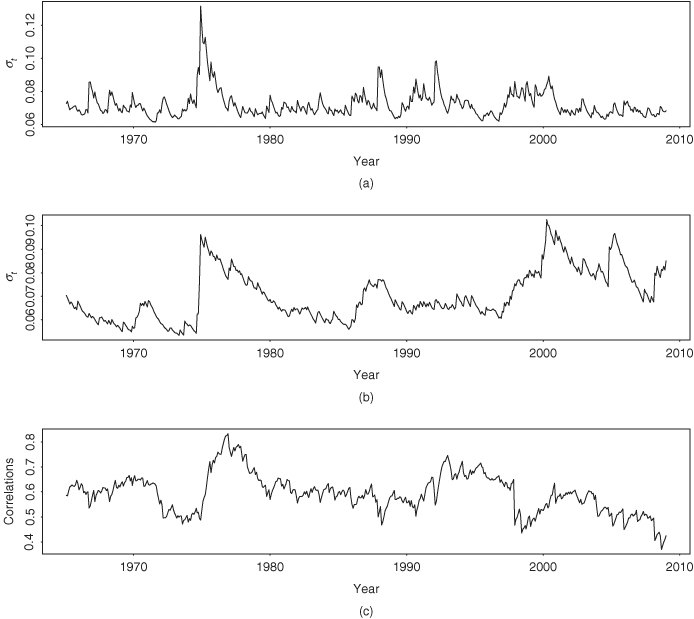
The output also provides some model checking statistics for individual stock returns. For instance, the Ljung–Box statistics for the standardized residual series and its squared series of Pfizer stock returns give Q(12) = 9.53(0.66) and Q(12) = 12.35(0.42), respectively, where the number in parentheses denotes the p value. Thus, checking the fitted model individually, one cannot reject the DVEC(1,1) model. A more informative model-checking approach is to apply the multivarite Q statistics to the bivariate standardized residual series and its squared process. Details are omitted. Interested readers are referred to Li (2004). Figure 10.5 shows the fitted volatility and correlation series. These series are stored in “sigma.t” and “R.t”, respectively. The correlations range from 0.37 to 0.83.
Figure 10.4 Time plot of monthly simple returns, including dividends, for Pfizer and Merck stocks from January 1965 to December 2008: (a) Pfizer stock and (b) Merck stock.

Figure 10.5 Estimated volatilities (standard error) and time-varying correlations of DVEC(1,1) model for monthly simple returns of two major drug companies from January 1965 to December 2008: (a) Pfizer stock volatility, (b) Merck stock volatility, and (c) time-varying correlations.
10.2.2 BEKK Model
To guarantee the positive-definite constraint, Engle and Kroner (1995) propose the Baba-Engle-Kraft-Kroner (BEKK) model,
10.6 ![]()
where ![]() is a lower triangular matrix and
is a lower triangular matrix and ![]() and
and ![]() are k × k matrices. Based on the symmetric parameterization of the model,
are k × k matrices. Based on the symmetric parameterization of the model, ![]() is almost surely positive definite provided that
is almost surely positive definite provided that ![]() is positive definite. This model also allows for dynamic dependence between the volatility series. On the other hand, the model has several disadvantages. First, the parameters in
is positive definite. This model also allows for dynamic dependence between the volatility series. On the other hand, the model has several disadvantages. First, the parameters in ![]() and
and ![]() do not have direct interpretations concerning lagged values of volatilities or shocks. Second, the number of parameters employed is k2(m + s) + k(k + 1)/2, which increases rapidly with m and s. Limited experience shows that many of the estimated parameters are statistically insignificant, introducing additional complications in modeling.
do not have direct interpretations concerning lagged values of volatilities or shocks. Second, the number of parameters employed is k2(m + s) + k(k + 1)/2, which increases rapidly with m and s. Limited experience shows that many of the estimated parameters are statistically insignificant, introducing additional complications in modeling.
Example 10.3
To illustrate, we consider the monthly simple returns of Pfizer and Merck stocks of Example 10.2 and employ a BEKK(1,1) model. Again, S-Plus is used to perform the estimation:
> mbekk=mgarch(rtn∼1,∼bekk(1,1))
> summary(mbekk)
Call:
mgarch(formula.mean = rtn ∼ 1, formula.var = ∼ bekk(1, 1))
Mean Equation: structure(.Data = rtn ∼ 1, class = "formula")
Conditional Var. Eq.: structure(.Data=∼bekk(1,1),
class="formula")
Conditional Distribution: gaussian
--------------------------------------------------------------
Estimated Coefficients:
--------------------------------------------------------------
Value Std.Error t value Pr(>|t|)
C(1) 1.329e-02 0.003247 4.094e+00 4.907e-05
C(2) 1.269e-02 0.003095 4.100e+00 4.792e-05
A(1, 1) 2.505e-02 0.008382 2.988e+00 2.938e-03
A(2, 1) 1.349e-02 0.004979 2.710e+00 6.946e-03
A(2, 2) 3.272e-06 8.453262 3.870e-07 1.000e+00
ARCH(1; 1, 1) 2.129e-01 0.084340 2.524e+00 1.190e-02
ARCH(1; 2, 1) 9.963e-02 0.072156 1.381e+00 1.680e-01
ARCH(1; 1, 2) 6.336e-02 0.076065 8.330e-01 4.052e-01
ARCH(1; 2, 2) 1.824e-01 0.062133 2.936e+00 3.467e-03
GARCH(1; 1, 1) 9.090e-01 0.063239 1.437e+01 0.000e+00
GARCH(1; 2, 1) -5.888e-02 0.047766 -1.233e+00 2.182e-01
GARCH(1; 1, 2) -8.231e-03 0.031512 -2.612e-01 7.940e-01
GARCH(1; 2, 2) 9.824e-01 0.022587 4.349e+01 0.000e+00
--------------------------------------------------------------
Ljung-Box test for standardized residuals:
--------------------------------------------------------------
Statistic P-value Chi^2-d.f.
pfe 9.465 0.6628 12
mrk 11.591 0.4791 12
Ljung-Box test for squared standardized residuals:
--------------------------------------------------------------
Statistic P-value Chi^2-d.f.
pfe 21.55 0.04291 12
mrk 9.19 0.68664 12
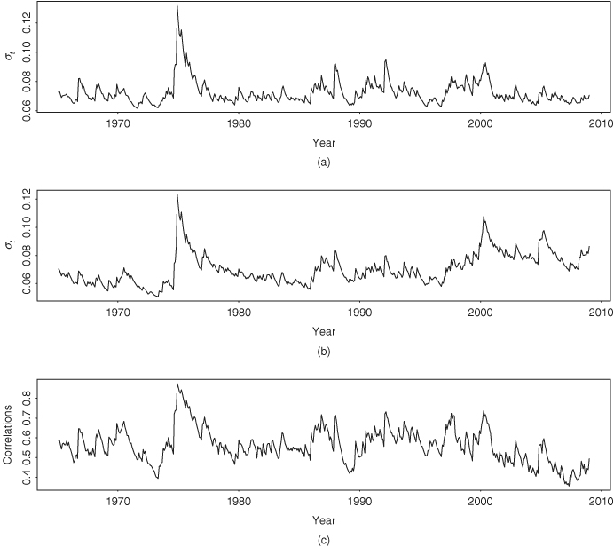
Model-checking statistics based on the individual residual series and provided by S-Plus fail to suggest any model inadequacy of the fitted BEKK(1,1) model. Figure 10.6 shows the fitted volatilities and the time-varying correlations of the BEKK(1,1) model. Compared with Figure 10.5, there are some differences between the two fitted volatility models. For instance, the time-varying correlations of the BEKK(1,1) model appear to be more volatile.
Figure 10.6 Estimated volatilities (standard error) and time-varying correlations of BEKK(1,1) model for monthly simple returns of two major drug companies from January 1965 to December 2008: (a) Pfizer stock volatility, (b) Merck stock volatility, and (c) time-varying correlations.
The volatility equation of the fitted BEKK(1,1) model is
where three estimates are insignificant at the 5% level. In general, the BEKK model tends to contain some insignificant parameter estimates, and one needs to perform matrix multiplication to decipher the fitted model.