
In this section, we consider some applications of the state-space model in finance and business. Our objectives are to highlight the applicability of the model and to demonstrate the practical implementation of the analysis in S-Plus with SsfPack.
Example
Consider the CAPM for the monthly simple excess returns of General Motors (GM) stock from January 1990 to December 2003; see Chapter 9. We use the simple excess returns of the S&P 500 composite index as the market returns. The returns are in percentages. Our illustration starts with a simple market model
11.86 ![]()
for t = 1, … , 168. This is a fixed-coefficient model and can easily be estimated by the ordinary least-squares (OLS) method. Denote the GM stock return and the market return by gm and sp, respectively. The result follows:
> da=read.table(“m-gmsp-excess-9003.txt”,header=F)
> gm=da[,1]
> sp=da[,2]
> fit=OLS(gm∼sp)
> summary(fit)
Call:
OLS(formula = gm∼sp)
Coefficients:
Value Std. Error t value Pr(>|t|)
(Intercept) 0.1982 0.6302 0.3145 0.7535
sp 1.0457 0.1453 7.1962 0.0000
Regression Diagnostics:
R-Squared 0.2378
Adjusted R-Squared 0.2332
Durbin-Watson Stat 2.0290
Residual Diagnostics:
Stat P-Value
Jarque-Bera 2.5348 0.2816
Ljung-Box 24.2132 0.3362
Residual standard error: 8.13 on 166 degrees of freedom
Thus, the fitted model is
![]()
Based on the residual diagnostics, the model appears to be adequate for the GM stock returns with adjusted R2 = 23.3%.
As shown in Section 11.3, model (11.86) is a special case of the state-space model. We then estimate the model using SsfPack. The result is as follows:
> reg.m=function(parm,mX=NULL){
+ parm=exp(parm) % log(sigma.e) is used to ensure positiveness.
+ ssf.reg=GetSsfReg(mX)
+ ssf.reg$mOmega[3,3]=parm[1]
+ CheckSsf(ssf.reg)
+ }
> c.start=c(10)
> X.mtx=cbind(rep(1,168),sp)
> reg.fit=SsfFit(c.start,gm,"reg.m",mX=X.mtx)
RELATIVE FUNCTION CONVERGENCE
> names(reg.fit)
[1] "parameters" "objective" "message" "grad.norm" "iterations"
[6] "f.evals" "g.evals" "hessian" "scale" "aux"
[11] "call" "vcov"
> sqrt(exp(reg.fit$parameters))
[1] 8.130114
> ssf.reg$mOmega[3,3]=exp(reg.fit$parameters)
> reg.s=SsfMomentEst(gm,ssf.reg,task="STSMO")
> reg.s$state.moment[10,]
state.1 state.2
0.1982025 1.045702
> sqrt(reg.s$state.variance[10,])
state.1 state.2
0.6302091 0.1453139
As expected, the result is in total agreement with that of the OLS method.
Finally, we entertain the time-varying CAPM of Section 11.3.1. The estimation result, including time plot of the smoothed response variable, is given below. The command SsfCondDens is used to compute the smoothed estimates of the state vector and observation without variance estimation.
> tv.capm =function(parm,mX=NULL){ %setup model for estimation
+ parm=exp(parm) %parameterize in log for positiveness.
+ Phi.t = rbind(diag(2),rep(0,2))
+ Omega=diag(parm)
+ JPhi=matrix(-1,3,2)
+ JPhi[3,1]=1
+ JPhi[3,2]=2
+ Sigma=-Phi.t
+ ssf.tv=list(mPhi=Phi.t,
+ mOmega=Omega,
+ mJPhi=JPhi,
+ mSigma=Sigma,
+ mX=mX)
+ CheckSsf(ssf.tv)
+ }
> tv.start=c(0,0,0) % starting values
> tv.mle=SsfFit(tv.start,gm,"tv.capm",mX=X.mtx) % estimation
> sigma.mle=sqrt(exp(tv.mle$parameters))
> sigma.mle
[1] 4.907845e-05 1.219885e-02 8.125213e+00
% Smoothing
> smoEst.tv=SsfCondDens(gm,tv.capm(tv.mle$parameters,mX=X.
mtx),
+ task="STSMO")
> names(smoEst.tv)
[1] "state" "response" "task"
> par(mfcol=c(2,2)) % plotting
> plot(gm,type='l',ylab='excess return')
> title(main='(a) Monthly simple excess returns')
> plot(smoEst.tv$response,type='l',ylab='rtn')
> title(main='(b) Expected returns')
> plot(smoEst.tv$state[,1],type='l',ylab='value')
> title(main='(c) Alpha(t)')
> plot(smoEst.tv$state[,2],type='l',ylab='value')
> title(main='(d) Beta(t)')
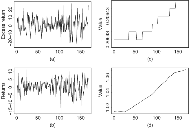
Note that estimates of ση and σε are 4.91 × 10⁻⁵ and 1.22 × 10⁻², respectively. These estimates are close to zero, indicating that αt and βt of the time-varying market model are essentially constant for the GM stock returns. This is in agreement with the fact that the fixed-coefficient market model fits the data well. Figure 11.5 shows some plots for the time-varying CAPM fit. Part (a) is the monthly simple excess returns of GM stock from January 1990 to December 2003. Part (b) is the expected returns of GM stock, that is, rt|T, where T = 168 is the sample size. Parts (c) and (d) are the time plots of the estimates of αt and βt. Given the tightness in the vertical scale, these two time plots confirm the assertion that a fixed-coefficient market model is adequate for the monthly GM stock return.
Figure 11.5 Time plots of some statistics for time-varying CAPM applied to monthly simple excess returns of General Motors stock. S&P 500 composite index return is used as market return: (a) monthly simple excess return, (b) expected returns rtIT, (c) αt estimate, and (d) βt estimate.
Example 11.3
In this example we reanalyze the series of quarterly earnings per share of Johnson & Johnson from 1960 to 1980 using the unobserved component model; see Chapter 2 for details of the data. The model considered is
11.87 ![]()
where yt is the logarithm of the observed earnings per share, μt is the local trend component satisfying
![]()
and γt is the seasonal component that satisfies
![]()
that is, ![]() . This model has three parameters—σe, ση, and σω—and is a simple unobserved component model. It can be put in a state-space form as
. This model has three parameters—σe, ση, and σω—and is a simple unobserved component model. It can be put in a state-space form as

where the covariance matrix of (ηt, ωt)′ is diag![]() , and yt = [1, 1, 0, 0]st + et; see Section 11.3. This is a special case of the structural time series in SsfPack and can easily be specified using the command GetSsfStsm. Performing the maximum-likelihood estimation, we obtain
, and yt = [1, 1, 0, 0]st + et; see Section 11.3. This is a special case of the structural time series in SsfPack and can easily be specified using the command GetSsfStsm. Performing the maximum-likelihood estimation, we obtain ![]()
> jnj=scan(file='q-jnj.txt')
> y=log(jnj)
% Estimation
> jnj.m=function(parm){
+ parm=exp(parm)
+ jnj.sea=GetSsfStsm(irregular=parm[1],level=parm[2],
+ seasonalDummy=c(parm[3],4))
+ CheckSsf(jnj.sea)
+ }
>
> c.start=c(0,0,0) % Starting values
> jnj.est=SsfFit(c.start,y,"jnj.m")
> names(jnj.est)
[1] "parameters" "objective" "message" "grad.norm" "iterations"
[6] "f.evals" "g.evals" "hessian" "scale" "aux"
[11] "call"
> jnjest=exp(jnj.est$parameters)
> jnjest % estimates
[1] 2.044516e-06 7.269655e-02 2.931691e-02
> jnj.ssf=GetSsfStsm(irregular=jnjest[1],level=jnjest[2],
+ seasonalDummy=c(jnjest[3],4)) % specify the model with estimates
> CheckSsf(jnj.ssf)
$mPhi:
[,1] [,2] [,3] [,4]
[1,] 1 0 0 0
[2,] 0 -1 -1 -1
[3,] 0 1 0 0
[4,] 0 0 1 0
[5,] 1 1 0 0
$mOmega:
[,1] [,2] [,3] [,4] [,5]
[1,] 0.005284788 0.000000000 0 0 0.000000e+00
[2,] 0.000000000 0.000859481 0 0 0.000000e+00
[3,] 0.000000000 0.000000000 0 0 0.000000e+00
[4,] 0.000000000 0.000000000 0 0 0.000000e+00
[5,] 0.000000000 0.000000000 0 0 4.180047e-12
$mSigma:
[,1] [,2] [,3] [,4]
[1,] -1 0 0 0
[2,] 0 -1 0 0
[3,] 0 0 -1 0
[4,] 0 0 0 -1
[5,] 0 0 0 0
$mDelta:
[,1]
[1,] 0
[2,] 0
[3,] 0
[4,] 0
[5,] 0
$mJPhi:
[1] 0
$mJOmega:
[1] 0
$mJDelta:
[1] 0
$mX:
[1] 0
$cT:
[1] 0
$cX:
[1] 0
$cY:
[1] 1
$cSt:
[1] 4
attr(, "class"):
[1] "ssf" % below: smoothed components
> jnj.smo=SsfMomentEst(y,jnj.ssf,task="STSMO")
> up1=jnj.smo$state.moment[,1]+
+ 2*sqrt(jnj.smo$state.variance[,1])
> lw1=jnj.smo$state.moment[,1]-
+ 2*sqrt(jnj.smo$state.variance[,1])
> max(up1) % obtain the range for plotting
[1] 2.795702
> min(lw1)
[1] -0.5948943
> up=jnj.smo$state.moment[,2]+
+ 2*sqrt(jnj.smo$state.variance[,2])
> lw=jnj.smo$state.moment[,2]-
+ 2*sqrt(jnj.smo$state.variance[,2])
> max(up)
[1] 0.3788652
> min(lw)
[1] -0.3552441
> par(mfcol=c(2,1)) % plotting
> plot(tdx,jnj.smo$state.moment[,1],type='l',xlab='year',
+ ylab='value',ylim=c(-1,3))
> lines(tdx,up1,lty=2)
> lines(tdx,lw1,lty=2)
> title(main='(a) Trend component')
> plot(tdx,jnj.smo$state.moment[,2],type='l',xlab='year',
+ ylab='value',ylim=c(-.5,.5))
> lines(tdx,up,lty=2)
> lines(tdx,lw,lty=2)
> title(main='(b) Seasonal component')
% Filtering and smoothing
> jnj.fil=KalmanFil(y,jnj.ssf,task="STFIL")
> jnj.smo1=KalmanSmo(jnj.fil,jnj.ssf)
> plot(tdx,jnj.fil$mOut[,1],type='l',xlab='year',ylab='resi')
> title(main='(a) 1-Step forecast error')
> plot(tdx,jnj.smo1$response.residuals[2:85],type='l',
+ xlab='year',ylab='resi')
> title(main='(b) Smoothing residual')
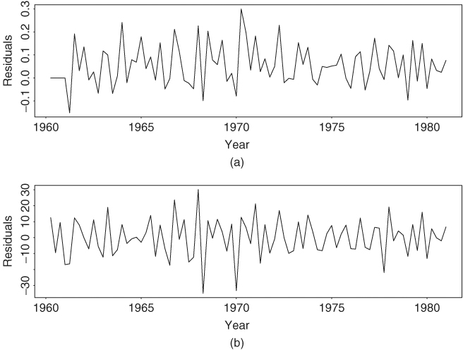
Figure 11.6 shows the smoothed estimates of the trend and seasonal components, that is, μt|T and γt|T with T = 84, of the data. Of particular interest is that the seasonal pattern seems to evolve over time. Also shown are 95% pointwise confidence regions of the unobserved components. Figure 11.7 shows the residual plots, where part (a) gives the 1-step-ahead forecast errors computed by Kalman filter and part (b) is the smoothed response residuals of the fitted model. Thus, state-space modeling provides an alternative approach for analyzing seasonal time series. It should be noted that the estimated components in Figure 11.6 are not unique. They depend on the model specified and constraints used. In fact, there are infinitely many ways to decompose an observed time series into unobserved components. For instance, one can use a different specification for the seasonal component, for example, sesonalTrig in SsfPack, to obtain another decomposition for the earnings series of Johnson & Johnson. Thus, care must be exercised in interpreting the estimated components. However, for forecasting purposes, the choice of decomposition does not matter provided that the chosen one is a valid decomposition.
Figure 11.6 Smoothed components of fitting model (11.87) to logarithm of quarterly earnings per share of Johnson & Johnson from 1960 to 1980: (a) trend component and (b) seasonal component. Dotted lines indicate pointwise 95% confidence regions.

Figure 11.7 Residual series of fitting model (11.87) to logarithm of quarterly earnings per share of Johnson & Johnson from 1960 to 1980: (a) 1-step-ahead forecast error vt and (b) smoothed residuals of response variable.
Exercises
11.1 Consider thar ARMA(1,1) model yt − 0.8yt−1 = at + 0.4at−1 with at ∼ N(0, 0.49). Convert the model into a state-space form using (a) Akaike's method, (b) Harvey's approach, and (c) Aoki's approach.
11.2 The file aa-rv-20m.txt contains the realized daily volatility series of Alcoa stock returns from January 2, 2003, to May 7, 2004; see the example in Section 11.1. The volatility series is constructed using 20-minute intradaily log returns.
a. Fit an ARIMA(0,1,1) model to the log volatility series and write down the model.
b. Estimate the local trend model in Eqs. (11.1) and (11.2) for the log volatility series. What are the estimates of σe and ση? Obtain time plots for the filtered and smoothed state variables with pointwise 95% confidence interval.
11.3 Consider the monthly simple excess returns of Pfizer stock and the S&P 500 composite index from January 1990 to December 2003. The excess returns are in m-pfesp-ex9003.txt with Pfizer stock returns in the first column.
a. Fit a fixed-coefficient market model to the Pfizer stock return. Write down the fitted model.
b. Fit a time-varying CAPM to the Pfizer stock return. What are the estimated standard errors of the innovations to the αt and βt series? Obtain time plots of the smoothed estimates of αt and βt.
11.4 Consider the AR(3) model
![]()
and suppose that the observed data are
![]()
where {et} and {at} are independent and the initial values of xj with j ≤ 0 are independent of et and at for t > 0.
a. Convert the model into a state-space form.
b. If E(et) = c, which is not zero, what is the corresponding state-space form for the system?
11.5 The file m-ppiaco4709.txt contains year, month, day, and U.S. producer price index (PPI) from January 1947 to November 2009. The index is for all commodities and not seasonally adjusted. Let zt = ln(Zt) − ln(Zt−1), where Zt is the observed monthly PPI. It turns out that an AR(3) model is adequate for zt if the minor seasonal dependence is ignored. Let yt be the sample mean-corrected series of zt.
a. Fit an AR(3) model to yt and write down the fitted model.
b. Suppose that yt has independent measurement errors so that yt = xt + et, where xt is a zero-mean AR(3) process and Var(et) = ![]() . Use a state-space form to estimate parameters, including the innovational variances to the state and
. Use a state-space form to estimate parameters, including the innovational variances to the state and ![]() . Write down the fitted model and obtain a time plot of the smoothed estimate of xt. Also, show the time plot of filtered response residuals of the fitted state-space model.
. Write down the fitted model and obtain a time plot of the smoothed estimate of xt. Also, show the time plot of filtered response residuals of the fitted state-space model.
Akaike, H.(1975).Markovian representation of stochastic processes by canonical variables. SIAM Journal on Control 13: 162–173.
Aoki, M.(1987). State Space Modeling of Time Series. Springer,New York.
Anderson, B. D. O. andMoore, J. B.(1979). Optimal Filtering. Prentice-Hall,Englewood Cliffs, NJ.
Chan, N. H.(2002). Time Series: Applications to Finance. Wiley,Hoboken, NJ.
de Jong, P.(1989).Smoothing and interpolation with the state space model. Journal of the American Statistical Association 84: 1085–1088.
Durbin, J. andKoopman, S. J.(2001). Time Series Analysis by State Space Methods. Oxford University Press,Oxford, UK.
Hamilton, J.(1994). Time Series Analysis. Princeton University Press,Princeton, NJ.
Harvey, A. C.(1993). Time Series Models, 2nd ed.Harvester Wheatsheaf,Hemel Hempstead, UK.
Kalman, R. E.(1960).A new approach to linear filtering and prediction problems. Journal of Basic Engineering, Transactions ASMA, Series D 82: 35–45.
Kim, C. J. andNelson, C. R.(1999). State Space Models with Regime Switching. Academic,New York.
Kitagawa, G. andGersch, W.(1996). Smoothness Priors Analysis of Time Series. Springer,New York.
Koopman, S. J.(1993).Disturbance smoother for state space models. Biometrika 80: 117–126.
Koopman, S. J.,Shephard, N., andDoornik, J. A.(1999).Statistical algorithms for models in state-space form using SsfPack 2.2. Econometrics Journal 2: 113–166. Also available athttp://www.ssfpack.com/.
Shumway, R. H. andStoffer, D. S.(2000). Time Series Analysis and Its Applications. Springer,New York.
West, M. andHarrison, J.(1997). Bayesian Forecasting and Dynamic Models, 2nd ed.Springer,New York.