2.7 Unit-Root Nonstationarity

So far we have focused on return series that are stationary. In some studies, interest rates, foreign exchange rates, or the price series of an asset are of interest. These series tend to be nonstationary. For a price series, the nonstationarity is mainly due to the fact that there is no fixed level for the price. In the time series literature, such a nonstationary series is called unit-root nonstationary time series. The best known example of unit-root nonstationary time series is the random-walk model.

2.7.1 Random Walk

A time series {pt} is a random walk if it satisfies

2.35

where p0 is a real number denoting the starting value of the process and {at} is a white noise series. If pt is the log price of a particular stock at date t, then p0 could be the log price of the stock at its initial public offering (IPO) (i.e., the logged IPO price). If at has a symmetric distribution around zero, then conditional on pt−1, pt has a 50–50 chance to go up or down, implying that pt would go up or down at random. If we treat the random-walk model as a special AR(1) model, then the coefficient of pt−1 is unity, which does not satisfy the weak stationarity condition of an AR(1) model. A random-walk series is, therefore, not weakly stationary, and we call it a unit-root nonstationary time series.

The random-walk model has widely been considered as a statistical model for the movement of logged stock prices. Under such a model, the stock price is not predictable or mean reverting. To see this, the 1-step-ahead forecast of model (2.35) at the forecast origin h is

which is the log price of the stock at the forecast origin. Such a forecast has no practical value. The 2-step-ahead forecast is

which again is the log price at the forecast origin. In fact, for any forecast horizon ℓ > 0, we have

Thus, for all forecast horizons, point forecasts of a random-walk model are simply the value of the series at the forecast origin. Therefore, the process is not mean reverting.

The MA representation of the random-walk model in Eq. (2.35) is

This representation has several important practical implications. First, the ℓ-step-ahead forecast error is

so that , which diverges to infinity as ℓ → ∞. The length of an interval forecast of ph+ℓ will approach infinity as the forecast horizon-increases. This result says that the usefulness of point forecast diminishes as ℓ increases, which again implies that the model is not predictable. Second, the unconditional variance of pt is unbounded because Var[eh(ℓ)] approaches infinity as ℓ increases. Theoretically, this means that pt can assume any real value for a sufficiently large t. For the log price pt of an individual stock, this is plausible. Yet for market indexes, negative log price is very rare if it happens at all. In this sense, the adequacy of a random-walk model for market indexes is questionable. Third, from the representation, ψi = 1 for all i. Thus, the impact of any past shock at−i on pt does not decay over time. Consequently, the series has a strong memory as it remembers all of the past shocks. In economics, the shocks are said to have a permanent effect on the series. The strong memory of a unit-root time series can be seen from the sample ACF of the observed series. The sample ACFs are all approaching 1 as the sample size increases.

2.7.2 Random Walk with Drift

As shown by empirical examples considered so far, the log return series of a market index tends to have a small and positive mean. This implies that the model for the log price is

2.36

where μ = E(pt − pt−1) and {at} is a zero-mean white noise series. The constant term μ of model (2.36) is very important in financial study. It represents the time trend of the log price pt and is often referred to as the drift of the model. To see this, assume that the initial log price is p0. Then we have

The last equation shows that the log price consists of a time trend tμ and a pure random-walk process . Because Var() = , where is the variance of at, the conditional standard deviation of pt is , which grows at a slower rate than the conditional expectation of pt. Therefore, if we graph pt against the time index t, we have a time trend with slope μ. A positive slope μ implies that the log price eventually goes to infinity. In contrast, a negative μ implies that the log price would converge to − ∞ as t increases. Based on the above discussion, it is then not surprising to see that the log return series of the CRSP value- and equal-weighted indexes have a small, but statistically significant, positive mean.

To illustrate the effect of the drift parameter on the price series, we consider the monthly log stock returns of the 3M Company from February 1946 to December 2008. As shown by the sample EACF in Table 2.5, the series has no significant serial correlation. The series thus follows the simple model

2.37

where 0.0103 is the sample mean of rt and has a standard error 0.0023. The mean of the monthly log returns of 3M stock is, therefore, significantly different from zero at the 1% level. As a matter of fact, the one-sample test of zero mean shows a t ratio of 4.44 with a p value close to 0. We use the log return series to construct two log price series, namely

where ai is the mean-corrected log return in Eq. (2.37) (i.e., at = rt − 0.0103). The pt is the log price of 3M stock, assuming that the initial log price is zero (i.e., the log price of January 1946 was zero). The is the corresponding log price if the mean of log returns was zero. Figure 2.10 shows the time plots of pt and as well as a straight line yt = 0.0103 × t + 1946, where t is the time sequence of the returns and 1946 is the starting year of the stock. From the plots, the importance of the constant 0.0103 in Eq. (2.37) is evident. In addition, as expected, it represents the slope of the upward trend of pt.

Figure 2.10 Time plots of log prices for 3M stock from February 1946 to December 2008, assuming that log price of January 1946 was zero. The “o” line is for log price without time trend. Straight line is yt = 0.0103 × t + 1946.

Interpretation of the Constant Term

From the previous discussions, it is important to understand the meaning of a constant term in a time series model. First, for an MA(q) model in Eq. (2.22), the constant term is simply the mean of the series. Second, for a stationary AR(p) model in Eq. (2.9) or ARMA(p, q) model in Eq. (2.28), the constant term is related to the mean via μ = ϕ0/(1 − ϕ1 − ⋯ − ϕp). Third, for a random walk with drift, the constant term becomes the time slope of the series. These different interpretations for the constant term in a time series model clearly highlight the difference between dynamic and usual linear regression models.

Another important difference between dynamic and regression models is shown by an AR(1) model and a simple linear regression model,

For the AR(1) model to be meaningful, the coefficient ϕ1 must satisfy |ϕ1| ≤ 1. However, the coefficient β1 can assume any fixed real number.

2.7.3 Trend-Stationary Time Series

A closely related model that exhibits linear trend is the trend-stationary time series model,

where rt is a stationary time series, for example, a stationary AR(p) series. Here pt grows linearly in time with rate β1 and hence can exhibit behavior similar to that of a random-walk model with drift. However, there is a major difference between the two models. To see this, suppose that p0 is fixed. The random-walk model with drift assumes the mean E(pt) = p0 + μt and variance Var(pt) = , both of them are time dependent. On the other hand, the trend-stationary model assumes the mean E(pt) = β0 + β1t, which depends on time, and variance Var(pt) = Var(rt), which is finite and time invariant. The trend-stationary series can be transformed into a stationary one by removing the time trend via a simple linear regression analysis. For analysis of trend-stationary time series, see the method of Section 2.9.

2.7.4 General Unit-Root Nonstationary Models

Consider an ARMA model. If one extends the model by allowing the AR polynomial to have 1 as a characteristic root, then the model becomes the well-known autoregressive integrated moving-average (ARIMA) model. An ARIMA model is said to be unit-root nonstationary because its AR polynomial has a unit root. Like a random-walk model, an ARIMA model has strong memory because the ψi coefficients in its MA representation do not decay over time to zero, implying that the past shock at−i of the model has a permanent effect on the series. A conventional approach for handling unit-root nonstationarity is to use differencing.

Differencing

A time series yt is said to be an ARIMA(p, 1, q) process if the change series ct = yt − yt−1 = (1 − B)yt follows a stationary and invertible ARMA(p, q) model. In finance, price series are commonly believed to be nonstationary, but the log return series, rt = ln(Pt) − ln(Pt−1), is stationary. In this case, the log price series is unit-root nonstationary and hence can be treated as an ARIMA process. The idea of transforming a nonstationary series into a stationary one by considering its change series is called differencing in the time series literature. More formally, ct = yt − yt−1 is referred to as the first differenced series of yt. In some scientific fields, a time series yt may contain multiple unit roots and needs to be differenced multiple times to become stationary. For example, if both yt and its first differenced series ct = yt − yt−1 are unit-root nonstationary, but st = ct − ct−1 = yt − 2yt−1 + yt−2 is weakly stationary, then yt has double unit roots, and st is the second differenced series of yt. In addition, if st follows an ARMA(p, q) model, then yt is an ARIMA(p, 2, q) process. For such a time series, if st has a nonzero mean, then yt has a quadratic time function and the quadratic time coefficient is related to the mean of st. The seasonally adjusted series of U.S. quarterly gross domestic product implicit price deflator might have double unit roots. However, the mean of the second differenced series is not significantly different from zero; see the Exercises of this chapter. Box, Jenkins, and Reinsel (1994) discuss many properties of general ARIMA models.

2.7.5 Unit-Root Test

To test whether the log price pt of an asset follows a random walk or a random walk with drift, we employ the models

2.38

2.39

where et denotes the error term, and consider the null hypothesis H0:ϕ1 = 1 versus the alternative hypothesis Ha:ϕ1 < 1. This is the well-known unit-root testing problem; see Dickey and Fuller (1979). A convenient test statistic is the t ratio of the least-squares (LS) estimate of ϕ1 under the null hypothesis. For Eq. (2.38), the LS method gives

where p0 = 0 and T is the sample size. The t ratio is

which is commonly referred to as the Dickey–Fuller (DF) test. If {et} is a white noise series with finite moments of order slightly greater than 2, then the DF statistic converges to a function of the standard Brownian motion as T → ∞; see Chan and Wei (1988) and Phillips (1987) for more information. If ϕ0 is zero but Eq. (2.39) is employed anyway, then the resulting t ratio for testing ϕ1 = 1 will converge to another nonstandard asymptotic distribution. In either case, simulation is used to obtain critical values of the test statistics; see Fuller (1976, Chapter 8) for selected critical values. Yet if ϕ0 ≠ 0 and Eq. (2.39) is used, then the t ratio for testing ϕ1 = 1 is asymptotically normal. However, large sample sizes are needed for the asymptotic normal distribution to hold. Standard Brownian motion is introduced in Chapter 6.

For many economic time series, ARIMA(p, d, q) models might be more appropriate than the simple model in Eq. (2.39). In the econometric literature, AR(p) models are often used. Denote the series by xt. To verify the existence of a unit root in an AR(p) process, one may perform the test H0:β = 1 vs. Ha:β < 1 using the regression

2.40

where ct is a deterministic function of the time index t and Δxj = xj − xj−1 is the differenced series of xt. In practice, ct can be zero or a constant or ct = ω0 + ω1t. The t ratio of ,

where denotes the least-squares estimate of β, is the well-known augmented Dickey–Fuller (ADF) unit-root test. Note that because of the first differencing, Eq. (2.40) is equivalent to an AR(p) model with deterministic function ct. Equation (2.40) can also be rewritten as

where βc = β − 1. One can then test the equivalent hypothesis H0:βc = 0 vs. Ha:βc < 0.

Example 2.2

Consider the log series of U.S. quarterly GDP from 1947.I to 2008.IV. The series exhibits an upward trend, showing the growth of the U.S. economy, and has high sample serial correlations; see the lower left panel of Figure 2.11. The first differenced series, representing the growth rate of U.S. GDP and also shown in Figure 2.11, seems to vary around a fixed mean level, even though the variability appears to be smaller in recent years. To confirm the observed phenomenon, we apply the ADF unit-root test to the log series. Based on the sample PACF of the differenced series shown in Figure 2.11, we choose p = 10. Other values of p are also used, but they do not alter the conclusion of the test. With p = 10, the ADF test statistic is − 1.701 with a p value 0.4297, indicating that the unit-root hypothesis cannot be rejected. From the attached S-Plus output, .

Figure 2.11 Log series of U.S. quarterly GDP from 1947.I to 2008.IV: (a) time plot of logged GDP series, (b) sample ACF of log GDP data, (c) time plot of first differenced series, and (d) sample PACF of differenced series.

R Demonstration

S-Plus Demonstration

The following output has been edited:

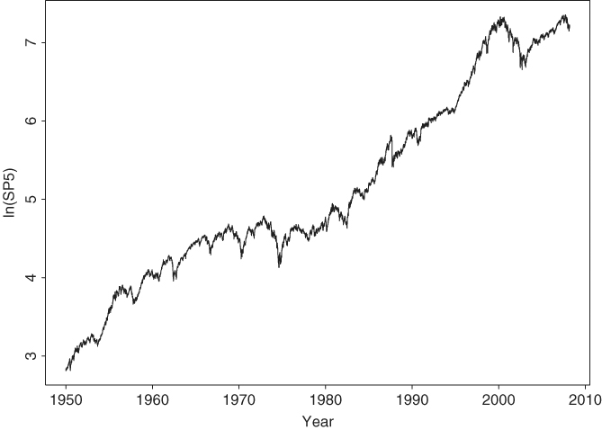
As another example, consider the log series of the S&P 500 index from January 3, 1950, to April 16, 2008, for 14,462 observations. The series is shown in Figure 2.12. Testing for a unit root in the index is relevant if one wishes to verify empirically that the Index follows a random walk with drift. To this end, we use ct = ω0 + ω1t in applying the ADF test. Furthermore, we choose p = 15 based on the sample PACF of the first differenced series. The resulting test statistic is − 1.998 with a p value 0.602. Thus, the unit-root hypothesis cannot be rejected at any reasonable significance level. The constant term is statistically significant, whereas the estimate of the time trend is not at the usual 5% level. The latter is significant at the 10% level, however. In summary, for the period from January 1950 to April 2008, the log series of the S&P 500 index contains a unit root and a positive drift, but there is no strong evidence of a time trend.

Figure 2.12 Time plot of logarithm of daily S&P 500 index from January 3, 1950, to April 16, 2008.

R Demonstration

S-Plus Demonstration

The following output has been edited: