2.8 Seasonal Models

Some financial time series such as quarterly earnings per share of a company exhibits certain cyclical or periodic behavior. Such a time series is called a seasonal time series. Figure 2.13(a) shows the time plot of quarterly earnings per share of Johnson & Johnson from the first quarter of 1960 to the last quarter of 1980. The data obtained from Shumway and Stoffer (2000) possess some special characteristics. In particular, the earnings grew exponentially during the sample period and had a strong seasonality. Furthermore, the variability of earnings increased over time. The cyclical pattern repeats itself every year so that the periodicity of the series is 4. If monthly data are considered (e.g., monthly sales of Wal-Mart stores), then the periodicity is 12. Seasonal time series models are also useful in pricing weather-related derivatives and energy futures because most environmental time series exhibit strong seasonal behavior.

Figure 2.13 Time plots of quarterly earnings per share of Johnson & Johnson from 1960 to 1980: (a) observed earnings and (b) log earnings.

Analysis of seasonal time series has a long history. In some applications, seasonality is of secondary importance and is removed from the data, resulting in a seasonally adjusted time series that is then used to make inference. The procedure to remove seasonality from a time series is referred to as seasonal adjustment. Most economic data published by the U.S. government are seasonally adjusted (e.g., the growth rate of gross domestic product and the unemployment rate). In other applications such as forecasting, seasonality is as important as other characteristics of the data and must be handled accordingly. Because forecasting is a major objective of financial time series analysis, we focus on the latter approach and discuss some econometric models that are useful in modeling seasonal time series.

2.8.1 Seasonal Differencing

Figure 2.13(b) shows the time plot of log earnings per share of Johnson & Johnson. We took the log transformation for two reasons. First, it is used to handle the exponential growth of the series. Indeed, the plot confirms that the growth is linear in the log scale. Second, the transformation is used to stablize the variability of the series. Again, the increasing pattern in variability of Figure 2.13(a) disappears in the new plot. Log transformation is commonly used in analysis of financial and economic time series. In this particular instance, all earnings are positive so that no adjustment is needed before taking the transformation. In some cases, one may need to add a positive constant to every data point before taking the transformation.

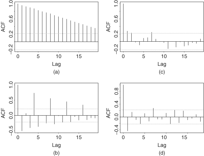
Denote the log earnings by xt. The upper left panel of Figure 2.14 shows the sample ACF of xt, which indicates that the quarterly log earnings per share has strong serial correlations. A conventional method to handle such strong serial correlations is to consider the first differenced series of xt [i.e., Δxt = xt − xt−1 = (1 − B)xt]. The lower left plot of Figure 2.14 gives the sample ACF of Δxt. The ACF is strong when the lag is a multiple of periodicity 4. This is a well-documented behavior of sample ACF of a seasonal time series. Following the procedure of Box, Jenkins, and Reinsel (1994, Chapter 9), we take another difference of the data, that is,

The operation Δ4 = (1 − B4) is called a seasonal differencing. In general, for a seasonal time series yt with periodicity s, seasonal differencing means

The conventional difference Δyt = yt − yt−1 = (1 − B)yt is referred to as the regular differencing. The lower right plot of Figure 2.14 shows the sample ACF of Δ4 Δxt, which has a significant negative ACF at lag 1 and a marginal negative correlation at lag 4. For completeness, Figure 2.14 also gives the sample ACF of the seasonally differenced series Δ4xt.

Figure 2.14 Sample ACF of log series of quarterly earnings per share of Johnson & Johnson from 1960 to 1980. (a) log earnings, (b) first differenced series, (c) seasonally differenced series, and (d) series with regular and seasonal differencing.

2.8.2 Multiplicative Seasonal Models

The behavior of the sample ACF of (1 − B4)(1 − B)xt in Figure 2.14 is common among seasonal time series. It led to the development of the following special seasonal time series model:

2.41

where s is the periodicity of the series, at is a white noise series, |θ| < 1, and |Θ| < 1. This model is referred to as the airline model in the literature; see Box, Jenkins, and Reinsel (1994, Chapter 9). It has been found to be widely applicable in modeling seasonal time series. The AR part of the model simply consists of the regular and seasonal differences, whereas the MA part involves two parameters. Focusing on the MA part (i.e., on the model),

where wt = (1 − Bs)(1 − B)xt and s > 1. It is easy to obtain that E(wt) = 0 and

Consequently, the ACF of the wt series is given by

and ρℓ = 0 for ℓ > 0 and ℓ ≠ 1, s − 1, s, s + 1. For example, if wt is a quarterly time series, then s = 4 and for ℓ > 0, the ACF ρℓ is nonzero at lags 1, 3, 4, and 5 only.

It is interesting to compare the prior ACF with those of the MA(1) model yt = (1 − θB)at and the MA(s) model zt = (1 − ΘBs)at. The ACF of yt and zt series are

We see that (i) ρ1 = ρ1(y), (ii) ρs = ρs(z), and (iii) ρs−1 = ρs+1 = ρ1(y) × ρs(z). Therefore, the ACF of wt at lags (s − 1) and (s + 1) can be regarded as the interaction between lag-1 and lag-s serial dependence, and the model of wt is called a multiplicative seasonal MA model. In practice, a multiplicative seasonal model says that the dynamics of the regular and seasonal components of the series are approximately orthogonal.

The model

2.42

where |θ| < 1 and |Θ| < 1, is a nonmultiplicative seasonal MA model. It is easy to see that for the model in Eq. (2.42), ρs+1 = 0. A multiplicative model is more parsimonious than the corresponding nonmultiplicative model because both models use the same number of parameters, but the multiplicative model has more nonzero ACFs.

Example 2.3

In this example we apply the airline model to the log series of quarterly earnings per share of Johnson & Johnson from 1960 to 1980. Based on the exact-likelihood method, the fitted model is

where standard errors of the two MA parameters are 0.080 and 0.101, respectively. The Ljung–Box statistics of the residuals show Q(12) = 10.0 with a p value of 0.44. The model appears to be adequate.

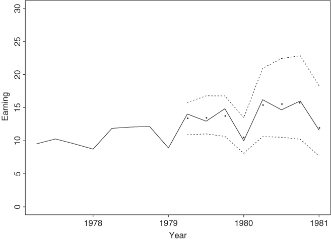
To illustrate the forecasting performance of the prior seasonal model, we reestimate the model using the first 76 observations and reserve the last 8 data points for forecasting evaluation. We compute 1-step- to 8-step-ahead forecasts and their standard errors of the fitted model at the forecast origin h = 76. An antilog transformation is taken to obtain forecasts of earnings per share using the relationship between normal and lognormal distributions given in Chapter 1. Figure 2.15 shows the forecast performance of the model, where the observed data are in solid line, point forecasts are shown by dots, and the dashed lines show 95% interval forecasts. The forecasts show a strong seasonal pattern and are close to the observed data. Finally, for an alternative approach to modeling the quarterly earnings data, see Example 11.3.

Figure 2.15 Out-of-sample point and interval forecasts for quarterly earnings of Johnson & Johnson. Forecast origin is fourth quarter of 1978. In plot, solid line shows actual observations, dots represent point forecasts, and dashed lines show 95% interval forecasts.

When the seasonal pattern of a time series is stable over time (e.g., close to a deterministic function), dummy variables may be used to handle the seasonality. This approach is taken by some analysts. However, deterministic seasonality is a special case of the multiplicative seasonal model discussed before. Specifically, if Θ = 1, then model (2.41) contains a deterministic seasonal component. Consequently, the same forecasts are obtained by using either dummy variables or a multiplicative seasonal model when the seasonal pattern is deterministic. Yet use of dummy variables can lead to inferior forecasts if the seasonal pattern is not deterministic. In practice, we recommend that the exact-likelihood method should be used to estimate a multiplicative seasonal model, especially when the sample size is small or when there is the possibility of having a deterministic seasonal component.

Example 2.4

To demonstrate deterministic seasonal behavior, consider the monthly simple returns of the CRSP Decile 1 Index from January 1970 to December 2008 for 468 observations. The series is shown in Figure 2.16(a), and the time plot does not show any clear pattern of seasonality. However, the sample ACF of the return series shown in Figure 2.16(b) contains significant lags at 12, 24, and 36 as well as lag 1. If seasonal ARMA models are entertained, a model in the form

is identified, where Rt denotes the monthly simple return. Using the conditional-likelihood method, the fitted model is

See the attached SCA (Scientific Computing Associates) output below. The estimates of the seasonal AR and MA coefficients are of similar magnitude. If the exact-likelihood method is used, we have

The cancellation between seasonal AR and MA factors is clearly seen. This highlights the usefulness of using the exact-likelihood method and, the estimation result suggests that the seasonal behavior might be deterministic. To further confirm this assertion, we define the dummy variable for January, that is,

and employ the simple linear regression

The fitted model is Rt = 0.0029 + 0.1253Jant + et, where the standard errors of the estimates are 0.0033 and 0.0115, respectively. The right panel of Figure 2.16 shows the time plot and sample ACF of the residual series of the prior simple linear regression. From the sample ACF, serial correlations at lags 12, 24, and 36 largely disappear, suggesting that the seasonal pattern of the Decile 1 returns has been successfully removed by the January dummy variable. Consequently, the seasonal behavior in the monthly simple return of Decile 1 is mainly due to the January effect.

Figure 2.16 Monthly simple returns of CRSP Decile 1 index from January 1970 to December 2008: (a) time plot of the simple returns, (b) sample ACF of simple returns, (c) time plot of simple returns after adjusting for January effect, and (d) sample ACF of adjusted simple returns.

R Demonstration

The following output has been edited and % denotes explanation:

SCA Demonstration

The following output has been edited: