
Although the ARCH model is simple, it often requires many parameters to adequately describe the volatility process of an asset return. For instance, consider the monthly excess returns of S&P 500 index of Example 3.3. An ARCH(9) model is needed for the volatility process. Some alternative model must be sought. Bollerslev (1986) proposes a useful extension known as the generalized ARCH (GARCH) model. For a log return series rt, let at = rt − μt be the innovation at time t. Then at follows a GARCH(m, s) model if
where again {ϵt} is a sequence of iid random variables with mean 0 and variance 1.0, α0 > 0, αi ≥ 0, βj ≥ 0, and ![]() . Here it is understood that αi = 0 for i > m and βj = 0 for j > s. The latter constraint on αi + βi implies that the unconditional variance of at is finite, whereas its conditional variance
. Here it is understood that αi = 0 for i > m and βj = 0 for j > s. The latter constraint on αi + βi implies that the unconditional variance of at is finite, whereas its conditional variance ![]() evolves over time. As before, ϵt is often assumed to follow a standard normal or standardized Student-t distribution or generalized error distribution. Equation (3.14) reduces to a pure ARCH(m) model if s = 0. The αi and βj are referred to as ARCH and GARCH parameters, respectively.
evolves over time. As before, ϵt is often assumed to follow a standard normal or standardized Student-t distribution or generalized error distribution. Equation (3.14) reduces to a pure ARCH(m) model if s = 0. The αi and βj are referred to as ARCH and GARCH parameters, respectively.
To understand properties of GARCH models, it is informative to use the following representation. Let ![]() so that
so that ![]() . By plugging
. By plugging ![]() =
= ![]() (i = 0, … , s) into Eq. (3.14), we can rewrite the GARCH model as
(i = 0, … , s) into Eq. (3.14), we can rewrite the GARCH model as
It is easy to check that {ηt} is a martingale difference series [i.e., E(ηt) = 0 and cov(ηt, ηt−j) = 0 for j ≥ 1]. However, {ηt} in general is not an iid sequence. Equation (3.15) is an ARMA form for the squared series ![]() . Thus, a GARCH model can be regarded as an application of the ARMA idea to the squared series
. Thus, a GARCH model can be regarded as an application of the ARMA idea to the squared series ![]() . Using the unconditional mean of an ARMA model, we have
. Using the unconditional mean of an ARMA model, we have
![]()
provided that the denominator of the prior fraction is positive.
The strengths and weaknesses of GARCH models can easily be seen by focusing on the simplest GARCH(1,1) model with
First, a large ![]() or
or ![]() gives rise to a large
gives rise to a large ![]() . This means that a large
. This means that a large ![]() tends to be followed by another large
tends to be followed by another large ![]() , generating, again, the well-known behavior of volatility clustering in financial time series. Second, it can be shown that if
, generating, again, the well-known behavior of volatility clustering in financial time series. Second, it can be shown that if ![]() , then
, then
![]()
Consequently, similar to ARCH models, the tail distribution of a GARCH(1,1) process is heavier than that of a normal distribution. Third, the model provides a simple parametric function that can be used to describe the volatility evolution.
Forecasts of a GARCH model can be obtained using methods similar to those of an ARMA model. Consider the GARCH(1,1) model in Eq. (3.16) and assume that the forecast origin is h. For 1-step-ahead forecast, we have
![]()
where ah and ![]() are known at the time index h. Therefore, the 1-step-ahead forecast is
are known at the time index h. Therefore, the 1-step-ahead forecast is
![]()
For multistep-ahead forecasts, we use ![]() and rewrite the volatility equation in Eq. (3.16) as
and rewrite the volatility equation in Eq. (3.16) as
![]()
When t = h + 1, the equation becomes
![]()
Since ![]() , the 2-step-ahead volatility forecast at the forecast origin h satisfies the equation
, the 2-step-ahead volatility forecast at the forecast origin h satisfies the equation
![]()
In general, we have
This result is exactly the same as that of an ARMA(1,1) model with AR polynomial 1 − (α1 + β1)B. By repeated substitutions in Eq. (3.17), we obtain that the ℓ-step-ahead forecast can be written as
![]()
Therefore,
![]()
provided that α1 + β1 < 1. Consequently, the multistep-ahead volatility forecasts of a GARCH(1,1) model converge to the unconditional variance of at as the forecast horizon increases to infinity provided that Var(at) exists.
The literature on GARCH models is enormous; see Bollerslev, Chou, and Kroner (1992), Bollerslev, Engle, and Nelson (1994), and the references therein. The model encounters the same weaknesses as the ARCH model. For instance, it responds equally to positive and negative shocks. In addition, recent empirical studies of high-frequency financial time series indicate that the tail behavior of GARCH models remains too short even with standardized Student-t innovations. For further information about kurtosis of GARCH models, see Section 3.16.
3.5.1 An Illustrative Example
The modeling procedure of ARCH models can also be used to build a GARCH model. However, specifying the order of a GARCH model is not easy. Only lower order GARCH models are used in most applications, say, GARCH(1,1), GARCH(2,1), and GARCH(1,2) models. The conditional maximum-likelihood method continues to apply provided that the starting values of the volatility ![]() are assumed to be known. Consider, for instance, a GARCH(1,1) model. If
are assumed to be known. Consider, for instance, a GARCH(1,1) model. If ![]() is treated as fixed, then
is treated as fixed, then ![]() can be computed recursively for a GARCH(1,1) model. In some applications, the sample variance of at serves as a good starting value of
can be computed recursively for a GARCH(1,1) model. In some applications, the sample variance of at serves as a good starting value of ![]() . The fitted model can be checked by using the standardized residual ãt = at/σt and its squared process.
. The fitted model can be checked by using the standardized residual ãt = at/σt and its squared process.
Example 3.3
In this example, we consider the monthly excess returns of S&P 500 index starting from 1926 for 792 observations. The series is shown in Figure 3.6. Denote the excess return series by rt. Figure 3.7 shows the sample ACF of rt and the sample PACF of ![]() . The rt series has some serial correlations at lags 1 and 3, but the key feature is that the PACF of
. The rt series has some serial correlations at lags 1 and 3, but the key feature is that the PACF of ![]() shows strong linear dependence. If an MA(3) model is entertained, we obtain
shows strong linear dependence. If an MA(3) model is entertained, we obtain
![]()
for the series, where all of the coefficients are significant at the 5% level. However, for simplicity, we use instead an AR(3) model
![]()
The fitted AR(3) model, under the normality assumption, is
For the GARCH effects, we use the GARCH(1,1) model
![]()
A joint estimation of the AR(3)–GARCH(1,1) model gives
![]()
From the volatility equation, the implied unconditional variance of at is
![]()
which is close to that of Eq. (3.18). However, t ratios of the parameters in the mean equation suggest that all three AR coefficients are insignificant at the 5% level. Therefore, we refine the model by dropping all AR parameters. The refined model is
The standard error of the constant in the mean equation is 0.0015, whereas those of the parameters in the volatility equation are 0.000024, 0.0197, and 0.0190, respectively. The unconditional variance of at is 0.000086/(1 − 0.8511 − 0.1216) = 0.00314. This is a simple stationary GARCH(1,1) model. Figure 3.8 shows the estimated volatility process, σt, and the standardized shocks ãt = at/σt for the GARCH(1,1) model in Eq. (3.19). The ãt series looks like a white noise process. Figure 3.9 provides the sample ACF of the standardized residuals ãt and the squared process ![]() . These ACFs fail to suggest any significant serial correlations or conditional heteroscedasticity in the standardized residual series. More specifically, we have Q(12) = 11.99(0.45) and Q(24) = 28.52(0.24) for ãt, and Q(12) = 13.11(0.36) and Q(24) = 26.45(0.33) for
. These ACFs fail to suggest any significant serial correlations or conditional heteroscedasticity in the standardized residual series. More specifically, we have Q(12) = 11.99(0.45) and Q(24) = 28.52(0.24) for ãt, and Q(12) = 13.11(0.36) and Q(24) = 26.45(0.33) for ![]() , where the number in parentheses is the p value of the test statistic. Thus, the model appears to be adequate in describing the linear dependence in the return and volatility series. Note that the fitted model shows
, where the number in parentheses is the p value of the test statistic. Thus, the model appears to be adequate in describing the linear dependence in the return and volatility series. Note that the fitted model shows ![]() = 0.9772, which is close to 1. This phenomenon is commonly observed in practice and it leads to imposing the constraint α1 + β1 = 1 in a GARCH(1,1) model, resulting in an integrated GARCH (or IGARCH) model; see Section 3.6.
= 0.9772, which is close to 1. This phenomenon is commonly observed in practice and it leads to imposing the constraint α1 + β1 = 1 in a GARCH(1,1) model, resulting in an integrated GARCH (or IGARCH) model; see Section 3.6.
Figure 3.6 Time series plot of monthly excess returns of S&P 500 index from 1926 to 1991.

Figure 3.7 (a) Sample ACF of monthly excess returns of S&P 500 index and (b) sample PACF of squared monthly excess returns. Sample period is from 1926 to 1991.
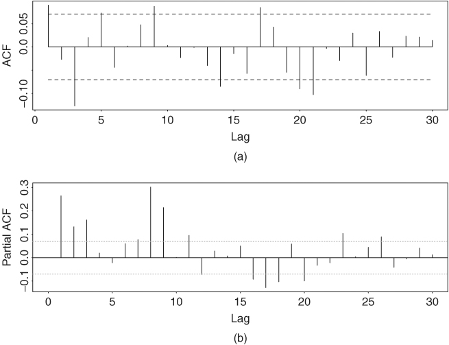
Figure 3.8 (a) Time series plot of estimated volatility (σt) for monthly excess returns of S&P 500 index and (b) standardized shocks of monthly excess returns of S&P 500 index. Both plots are based on GARCH(1,1) model in Eq. (3.19).
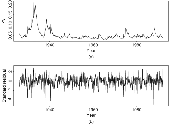
Figure 3.9 Model checking of GARCH(1,1) model in Eq. (3.19) for monthly excess returns of S&P 500 index: (a) Sample ACF of standardized residuals and (b) sample ACF of the squared standardized residuals.

Finally, to forecast the volatility of monthly excess returns of the S&P 500 index, we can use the volatility equation in Eq. (3.19). For instance, at the forecast origin h, we have ![]() . The 1-step-ahead forecast is then
. The 1-step-ahead forecast is then
![]()
where ah is the residual of the mean equation at time h and σh is obtained from the volatility equation. The starting value ![]() is fixed at either zero or the unconditional variance of at. For multistep-ahead forecasts, we use the recursive formula in Eq. (3.17). Table 3.1 shows some mean and volatility forecasts for the monthly excess return of the S&P 500 index with forecast origin h = 792 based on the GARCH(1,1) model in Eq. (3.19).
is fixed at either zero or the unconditional variance of at. For multistep-ahead forecasts, we use the recursive formula in Eq. (3.17). Table 3.1 shows some mean and volatility forecasts for the monthly excess return of the S&P 500 index with forecast origin h = 792 based on the GARCH(1,1) model in Eq. (3.19).
Table 3.1 Volatility Forecasts for Monthly Excess Returns of S&P 500 Indexa
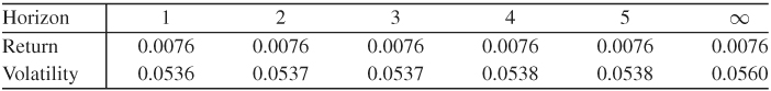
aThe forecast origin is h = 792, which corresponds to December 1991. Here volatility denotes conditional standard deviation.
Some S-Plus Commands Used in Example 3.3
> fit=garch(sp∼ar(3),∼garch(1,1))
> summary(fit)
> fit=garch(sp∼1,∼garch(1,1))
> summary(fit)
> names(fit)
[1] “residuals” “sigma.t” “df.residual” “coef” “model”
[6] “cond.dist” “likelihood” “opt.index” “cov”
“prediction”
[11] “call” “asymp.sd” “series”
>
> stdresi=fit$residuals/fit$sigma.t
> autocorTest(stdresi,lag=24)
> autocorTest(stdresiˆ2,lag=24)
> predict(fit,5)
Note that in the prior commands the volatility series σt is stored in fit$sigma.t and the residual series of the returns in fit$residuals.
t Innovation
Assuming that ϵt follows a standardized Student-t distribution with 5 degrees of freedom, we reestimate the GARCH(1,1) model and obtain
where the standard errors of the parameters are 0.0015, 0.51 × 10⁻⁴, 0.0296, and 0.0371, respectively. This model is essentially an IGARCH(1,1) model as ![]() ≈ 0.95, which is close to 1. The Ljung–Box statistics of the standardized residuals give Q(10) = 11.38 with a p value of 0.33 and those of the
≈ 0.95, which is close to 1. The Ljung–Box statistics of the standardized residuals give Q(10) = 11.38 with a p value of 0.33 and those of the ![]() series give Q(10) = 10.48 with a p value of 0.40. Thus, the fitted GARCH(1,1) model with Student-t distribution is adequate.
series give Q(10) = 10.48 with a p value of 0.40. Thus, the fitted GARCH(1,1) model with Student-t distribution is adequate.
S-Plus Commands Used
> fit1 = garch(sp∼1,∼garch(1,1),cond.dist=‘t’,cond.par=5,
+ cond.est=F)
> summary(fit1)
> stresi=fit1$residuals/fit1$sigma.t
> autocorTest(stresi,lag=10)
> autocorTest(stresiˆ2,lag=10)
Estimation of Degrees of Freedom
If we further extend the GARCH(1,1) model by estimating the degrees of freedom of the Student-t distribution used, we obtain the model
where the estimated degrees of freedom is 7.02. Standard errors of the estimates in Eq. (3.21) are close to those in Eq. (3.20). The standard error of the estimated degrees of freedom is 1.78. Consequently, we cannot reject the hypothesis of using a standardized Student-t distribution with 5 degrees of freedom at the 5% significance level.
S-Plus Commands Used
> fit2 = garch(sp∼1,∼garch(1,1),cond.dist=‘t’)
> summary(fit2)
R Commands Used in Example 3.3
> library(fGarch)
> sp5=scan(file=‘sp500.txt’) % Load data
> plot(sp5,type=‘l’)
% Below, fit an AR(3)+GARCH(1,1) model.
> m1=garchFit(∼arma(3,0)+garch(1,1),data=sp5,trace=F)
> summary(m1)
% Below, fit a GARCH(1,1) model with Student-t distribution.
> m2=garchFit(∼garch(1,1),data=sp5,trace=F,cond.dist=“std”)
> summary(m2)
% Obtain standardized residuals.
> stresi=residuals(m2,standardize=T)
> plot(stresi,type=‘l’)
> Box.test(stresi,10,type=‘Ljung’)
> predict(m2,5)
3.5.2 Forecasting Evaluation
Since the volatility of an asset return is not directly observable, comparing the forecasting performance of different volatility models is a challenge to data analysts. In the literature, some researchers use out-of-sample forecasts and compare the volatility forecasts ![]() with the shock
with the shock ![]() in the forecasting sample to assess the forecasting performance of a volatility model. This approach often finds a low correlation coefficient between
in the forecasting sample to assess the forecasting performance of a volatility model. This approach often finds a low correlation coefficient between ![]() and
and ![]() , that is, low R2. However, such a finding is not surprising because
, that is, low R2. However, such a finding is not surprising because ![]() alone is not an adequate measure of the volatility at time index h + ℓ. Consider the 1-step-ahead forecasts. From a statistical point of view,
alone is not an adequate measure of the volatility at time index h + ℓ. Consider the 1-step-ahead forecasts. From a statistical point of view, ![]() =
= ![]() so that
so that ![]() is a consistent estimate of
is a consistent estimate of ![]() . But it is not an accurate estimate of
. But it is not an accurate estimate of ![]() because a single observation of a random variable with a known mean value cannot provide an accurate estimate of its variance. Consequently, such an approach to evaluate forecasting performance of volatility models is strictly speaking not proper. For more information concerning forecasting evaluation of GARCH models, readers are referred to Andersen and Bollerslev (1998).
because a single observation of a random variable with a known mean value cannot provide an accurate estimate of its variance. Consequently, such an approach to evaluate forecasting performance of volatility models is strictly speaking not proper. For more information concerning forecasting evaluation of GARCH models, readers are referred to Andersen and Bollerslev (1998).
3.5.3 A Two-Pass Estimation Method
Based on Eq. (3.15), a two-pass estimation method can be used to estimate GARCH models. First, ignoring any ARCH effects, one estimates the mean equation of a return series using the methods discussed in Chapter 2 (e.g., maximum-likelihood method). Denote the residual series by at. Second, treating ![]() as an observed time series, one applies the maximum-likelihood method to estimate parameters of Eq. (3.15). Denote the AR and MA coefficient estimates by
as an observed time series, one applies the maximum-likelihood method to estimate parameters of Eq. (3.15). Denote the AR and MA coefficient estimates by ![]() and
and ![]() . The GARCH estimates are obtained as
. The GARCH estimates are obtained as ![]() and
and ![]() . Obviously, such estimates are approximations to the true parameters and their statistical properties have not been rigorously investigated. However, limited experience shows that this simple approach often provides good approximations, especially when the sample size is moderate or large. For instance, consider the monthly excess return series of the S&P 500 index of Example 3.3. Using the conditional MLE method in SCA, we obtain the model
. Obviously, such estimates are approximations to the true parameters and their statistical properties have not been rigorously investigated. However, limited experience shows that this simple approach often provides good approximations, especially when the sample size is moderate or large. For instance, consider the monthly excess return series of the S&P 500 index of Example 3.3. Using the conditional MLE method in SCA, we obtain the model
![]()
where all estimates are significantly different from zero at the 5% level. From the estimates, we have ![]() and
and ![]() . These approximate estimates are very close to those in Eq. (3.19) or (3.21). Furthermore, the fitted volatility series of the two-pass method is very close to that of Figure 3.8(a).
. These approximate estimates are very close to those in Eq. (3.19) or (3.21). Furthermore, the fitted volatility series of the two-pass method is very close to that of Figure 3.8(a).