
In finance, when using continuous-time models, it is common to assume that the price of an asset is an Ito process. Therefore, to derive the price of a financial derivative, one needs to use Ito's calculus. In this section, we briefly review Ito's lemma by treating it as a natural extension of the differentiation in calculus. Ito's lemma is the basis of stochastic calculus.
6.3.1 Review of Differentiation
Let G(x) be a differentiable function of x. Using the Taylor expansion, we have
![]()
Taking the limit as Δx → 0 and ignoring the higher order terms of Δx, we have
![]()
When G is a function of x and y, we have
![]()
Taking the limit as Δx → 0 and Δy → 0, we have
![]()
6.3.2 Stochastic Differentiation
Turn next to the case in which G is a differentiable function of xt and t, and xt is an Ito process. The Taylor expansion becomes
A discretized version of the Ito process is
where, for simplicity, we omit the arguments of μ and σ, and Δx = xt+Δt − xt. From Eq. (6.4), we have
where H(Δt) denotes higher order terms of Δt. This result shows that (Δx)2 contains a term of order Δt, which cannot be ignored when we take the limit as Δt → 0. However, the first term on the right-hand side of Eq. (6.5) has some nice properties:
![]()
where we use E(ϵ4) = 3 for a standard normal random variable. These two properties show that σ2ϵ2 Δt converges to a nonstochastic quantity σ2 Δt as Δt → 0. Consequently, from Eq. (6.5), we have
![]()
Plugging the prior result into Eq. (6.3) and using Ito's equation of xt in Eq. (6.2), we obtain
which is the well-known Ito lemma in stochastic calculus.
Recall that we suppressed the argument (xt, t) from the drift and volatility terms μ and σ in the derivation of Ito's lemma. To avoid any possible confusion in the future, we restate the lemma as follows.
Ito's Lemma
Assume that xt is a continuous-time stochastic process satisfying
![]()
where wt is a Wiener process. Furthermore, G(xt, t) is a differentiable function of xt and t. Then,
(6.6) ![]()
Example 6.1
As a simple illustration, consider the square function ![]() of the Wiener process. Here we have μ(wt, t) = 0, σ(wt, t) = 1, and
of the Wiener process. Here we have μ(wt, t) = 0, σ(wt, t) = 1, and
![]()
Therefore,
6.3.3 An Application
Let Pt be the price of a stock at time t, which is continuous in [0, ∞). In the literature, it is common to assume that Pt follows the special Ito process
where μ and σ are constant. Using the notation of the general Ito process in Eq. (6.2), we have μ(xt, t) = μxt and σ(xt, t) = σxt, where xt = Pt. Such a special process is referred to as a geometric Brownian motion. We now apply Ito's lemma to obtain a continuous-time model for the logarithm of the stock price Pt. Let G(Pt, t) = ln(Pt) be the log price of the underlying stock. Then we have
![]()
Consequently, via Ito's lemma, we obtain
This result shows that the logarithm of a price follows a generalized Wiener process with drift rate μ − σ2/2 and variance rate σ2 if the price is a geometric Brownian motion. Consequently, the change in logarithm of price (i.e., log return) between current time t and some future time T is normally distributed with mean (μ − σ2/2)(T − t) and variance σ2(T − t). If the time interval T − t = Δ is fixed and we are interested in equally spaced increments in log price, then the increment series is a Gaussian process with mean (μ − σ2/2) Δ and variance σ2 Δ.
6.3.4 Estimation of μ and σ
The two unknown parameters μ and σ of the geometric Brownian motion in Eq. (6.8) can be estimated empirically. Assume that we have n + 1 observations of stock price Pt at equally spaced time interval Δ (e.g., daily, weekly, or monthly). We measure Δ in years. Denote the observed prices as {P0, P1, … , Pn} and let rt = ln(Pt) − ln(Pt−1) for t = 1, … , n.
Since Pt = Pt−1exp(rt), rt is the continuously compounded return in the tth time interval. Using the result of the previous section and assuming that the stock price Pt follows a geometric Brownian motion, we obtain that rt is normally distributed with mean (μ − σ2/2) Δ and variance σ2 Δ. In addition, the rt are not serially correlated.
For simplicity, define μr = E(rt) = (μ − σ2/2) Δ and ![]() . Let
. Let ![]() and sr be the sample mean and standard deviation of the data—that is,
and sr be the sample mean and standard deviation of the data—that is,

As mentioned in Chapter 1, ![]() and sr are consistent estimates of the mean and standard deviation of ri, respectively. That is, → μr and sr → σr as n → ∞. Therefore, we may estimate σ by
and sr are consistent estimates of the mean and standard deviation of ri, respectively. That is, → μr and sr → σr as n → ∞. Therefore, we may estimate σ by
![]()
Furthermore, it can be shown that the standard error of this estimate is approximately ![]() . From
. From ![]() , we can estimate μ by
, we can estimate μ by
![]()
When the series rt is serially correlated or when the price of the asset does not follow the geometric Brownian motion in Eq. (6.8), then other estimation methods must be used to estimate the drift and volatility parameters of the diffusion equation. We return to this issue later.
Example 6.2
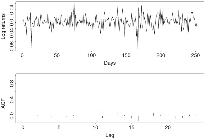
Consider the daily log returns of IBM stock in 1998. Figure 6.2(a) shows the time plot of the data, which have 252 observations. Figure 6.2(b) shows the sample autocorrelations of the series. It is seen that the log returns are indeed serially uncorrelated. The Ljung–Box statistic gives Q(10) = 4.9, which is highly insignificant compared with a chi-squared distribution with 10 degrees of freedom.
Figure 6.2 Daily returns of IBM stock in 1998: (a) log returns and (b) sample autocorrelations.
If we assume that the price of IBM stock in 1998 follows the geometric Brownian motion in Eq. (6.8), then we can use the daily log returns to estimate the parameters μ and σ. From the data, we have ![]() and sr = 0.01915. Since 1 trading day is equivalent to Δ = 1/252 year, we obtain that
and sr = 0.01915. Since 1 trading day is equivalent to Δ = 1/252 year, we obtain that
![]()
Thus, the estimated expected return was 61.98% and the standard deviation was 30.4% per annum for IBM stock in 1998.
The normality assumption of the daily log returns may not hold, however. In this particular instance, the skewness − 0.464(0.153) and excess kurtosis 2.396(0.306) raise some concern, where the number in parentheses denotes asymptotic standard error.
Example 6.3
Consider the daily log return of the stock of Cisco Systems, Inc. in 2007. There are 251 observations, and the sample mean and standard deviation are − 3.81 × 10⁻⁵ and 0.0174, respectively. The log return series also shows no serial correlation with Q(12) = 12.30 with a p value of 0.42. Therefore, we have
![]()
Consequently, the estimated expected log return for Cisco Systems' stock was − 0.94% per annum, and the estimated standard deviation was 27.5% per annum in 2007.