5.4 Models for Price Changes

The discreteness and concentration on “no change” make it difficult to model the intraday price changes. Campbell et al. (1997) discuss several econometric models that have been proposed in the literature. Here we mention two models that have the advantage of employing explanatory variables to study the intraday price movements. The first model is the ordered probit model used by Hauseman, Lo, and MacKinlay (1992) to study the price movements in transactions data. The second model has been considered recently by McCulloch and Tsay (2000) and is a simplified version of the model proposed by Rydberg and Shephard (2003); see also Ghysels (2000).

5.4.1 Ordered Probit Model

Let be the unobservable price change of the asset under study (i.e., ), where is the virtual price of the asset at time t. The ordered probit model assumes that is a continuous random variable and follows the model

5.15

where xi is a p-dimensional row vector of explanatory variables available at time ti−1, β is a p × 1 parameter vector, E(ϵi|xi) = 0, Var(ϵi|xi) = , and Cov(ϵi, ϵj) = 0 for i ≠ j. The conditional variance is assumed to be a positive function of the explanatory variable wi, that is,

5.16

where g( · ) is a positive function. For financial transactions data, wi may contain the time interval ti − ti−1 and some conditional heteroscedastic variables. Typically, one also assumes that the conditional distribution of ϵi given xi and wi is Gaussian.

Suppose that the observed price change yi may assume k possible values. In theory, k can be infinity, but countable. In practice, k is finite and may involve combining several categories into a single value. For example, we have k = 7 in Table 5.1, where the first value “ − 3 ticks” means that the price change is − 3 ticks or lower. We denote the k possible values as {s1, … , sk}. The ordered probit model postulates the relationship between yi and as

5.17

where αj are real numbers satisfying − ∞ = α0 < α1 < ⋯ < αk−1 < αk = ∞. Under the assumption of conditional Gaussian distribution, we have

5.18

where Φ(x) is the cumulative distribution function of the standard normal random variable evaluated at x, and we write σi(wi) to denote that is a positive function of wi. From the definition, an ordered probit model is driven by an unobservable continuous random variable. The observed values, which have a natural ordering, can be regarded as categories representing the underlying process.

The ordered probit model contains parameters β, αi (i = 1, … , k − 1), and those in the conditional variance function σi(wi) in Eq. (5.16). These parameters can be estimated by the maximum-likelihood or Markov chain Monte Carlo methods.

The parameter estimates and their t ratios are given in Table 5.5. All the t ratios are large except one, indicating that the estimates are highly significant. Such high t ratios are not surprising as the sample size is large. For the heavily traded IBM stock, the estimation results suggest the following conclusions:

Table 5.5 Parameter Estimates of Ordered Probit Model in Eqs. (5.19) and (5.20) for the 1988 Transaction Data of IBM, Where t Denotes the t Ratio

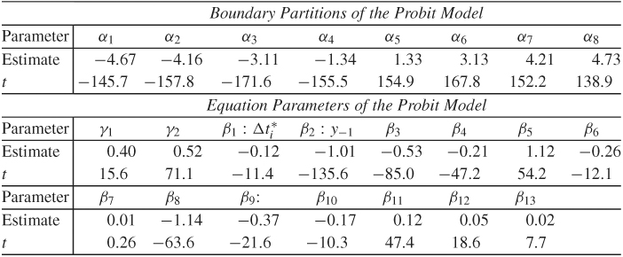
Source: Reprinted with permission of Elsevier from Journal of Financial Economics (1992, Vol. 31, p. 345)

5.4.2 Decomposition Model

An alternative approach to modeling price change is to decompose it into three components and use conditional specifications for the components; see Rydberg and Shephard (2003). The three components are an indicator for price change, the direction of price movement if there is a change, and the size of price change if a change occurs. Specifically, the price change at the ith transaction can be written as

5.21

where Ai is a binary variable defined as

5.22

Di is also a discrete variable signifying the direction of the price change if a change occurs, that is,

5.23

where Di|(Ai = 1) means that Di is defined under the condition of Ai = 1, and Si is the size of the price change in ticks if there is a change at the ith trade and Si = 0 if there is no price change at the ith trade. When there is a price change, Si is a positive integer-valued random variable.

Note that Di is not needed when Ai = 0, and there is a natural ordering in the decomposition. Di is well defined only when Ai = 1 and Si is meaningful when Ai = 1 and Di is given. Model specification under the decomposition makes use of the ordering.

Let Fi be the information set available at the ith transaction. Examples of elements in Fi are Δti−j, Ai−j, Di−j, and Si−j for j ≥ 0. The evolution of price change under model (5.21) can then be partitioned as

5.24

Since Ai is a binary variable, it suffices to consider the evolution of the probability pi = P(Ai = 1) over time. We assume that

5.25

where xi is a finite-dimensional vector consisting of elements of Fi−1 and β is a parameter vector. Conditioned on Ai = 1, Di is also a binary variable, and we use the following model for δi = P(Di = 1|Ai = 1):

5.26

where zi is a finite-dimensional vector consisting of elements of Fi−1 and γ is a parameter vector. To allow for asymmetry between positive and negative price changes, we assume that

5.27

where g(λ) is a geometric distribution with parameter λ and the parameters λj, i evolve over time as

5.28

where wi is again a finite-dimensional explanatory variable in Fi−1 and θj is a parameter vector.

In Eq. (5.27), the probability mass function of a random variable x, which follows the geometric distribution g(λ), is

We added 1 to the geometric distribution so that the price change, if it occurs, is at least 1 tick. In Eq. (5.28), we take the logistic transformation to ensure that λj, i ∈ [0, 1].

The previous specification classifies the ith trade, or transaction, into one of three categories:

Let Ii(j) for j = 1, 2, 3 be the indicator variables of the prior three categories. That is, Ii(j) = 1 if the jth category occurs and Ii(j) = 0 otherwise. The log-likelihood function of Eq. (5.24) becomes

and the overall log-likelihood function is

5.29

which is a function of parameters β, γ, θu, and θd.

Example 5.2

We illustrate the decomposition model by analyzing the intraday transactions of IBM stock from November 1, 1990, to January 31, 1991. There were 63 trading days and 59,838 intraday transactions in the normal trading hours. The explanatory variables used are:

1. Ai−1: the action indicator of the previous trade [i.e., the (i − 1)th trade within a trading day]

2. Di−1: the direction indicator of the previous trade

3. Si−1: the size of the previous trade

4. Vi−1: the volume of the previous trade, divided by 1000

5. Δti−1: time duration from the (i − 2)th to (i − 1)th trade

6. BAi: the bid–ask spread prevailing at the time of transaction

Because we use lag-1 explanatory variables, the actual sample size is 59,775. It turns out that Vi−1, Δti−1, and BAi are not statistically significant for the model entertained. Thus, only the first three explanatory variables are used. The model employed is

5.30

The parameter estimates, using the log-likelihood function in Eq. (5.29), are given in Table 5.6. The estimated simple model shows some dynamic dependence in the price change. In particular, the trade-by-trade price changes of IBM stock exhibit some appealing features:

1. The probability of a price change depends on the previous price change. Specifically, we have

The result indicates that a price change may occur in clusters and, as expected, most transactions are without price change. When no price change occurred at the (i − 1)th trade, then only about one out of four trades in the subsequent transaction has a price change. When there is a price change at the (i − 1)th transaction, the probability of a price change in the ith trade increases to about 0.5.

2. The direction of price change is governed by

This result says that (a) if no price change occurred at the (i − 1)th trade, then the chances for a price increase or decrease at the ith trade are about even; and (b) the probabilities of consecutive price increases or decreases are very low. The probability of a price increase at the ith trade given that a price change occurs at the ith trade and there was a price increase at the (i − 1)th trade is only 8.6%. However, the probability of a price increase is about 90% given that a price change occurs at the ith trade and there was a price decrease at the (i − 1)th trade. Consequently, this result shows the effect of bid–ask bounce and supports price reversals in high-frequency trading.

3. There is weak evidence suggesting that big price changes have a higher probability to be followed by another big price change. Consider the size of a price increase. We have

Using the probability mass function of a geometric distribution, we obtain that the probability of a price increase by one tick is 0.827 at the ith trade if the transaction results in a price increase and Si−1 = 1. The probability reduces to 0.709 if Si−1 = 2 and to 0.556 if Si−1 = 3. Consequently, the probability of a large Si is proportional to Si−1 given that there is a price increase at the ith trade.

Table 5.6 Parameter Estimates of ADS Model in Eq. (5.30) for IBM Intraday Transactions from December 1, 1990, to January 31, 1991

A difference between the ADS of Eq. (5.21) and ordered probit models is that the former does not require any truncation or grouping in the size of a price change.

R Demonstration for Logistic Linear Regression

The following output has been edited: