
In several important locations in Excel, you can control the way your worksheets appear on the screen. These include the View tab on the ribbon, shown in Figure 3-21, and the General and Advanced categories in the Excel Options dialog box. Some options, such as Gridline Color, are self-explanatory; here we’ll talk about options with “issues.”
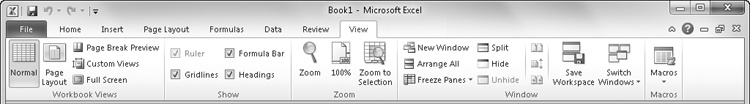
Figure 3-21. The View tab on the ribbon contains commands you can use to control the appearance of your workbook.
The Show group on the View tab controls the display of the formula bar as well as the appearance of gridlines, column and row headings, and the ruler (which is active only in Page Layout view). These are the options that are most often used, which is why they appear on the ribbon. But you’ll discover more ways to tweak your UI when you click the File menu and then click Excel Options.
Note
For more about Page Layout view, see Chapter 11. For more about security issues, see Chapter 4.
The Advanced category in the Excel Options dialog box contains three groups of options, shown in Figure 3-22 (you’ll need to scroll down a bit), that control different display behaviors for the program in general and for workbooks and worksheets in particular.

Figure 3-22. The Advanced category in the Excel Options dialog box includes a number of display options.
The Display area, shown scrolled to the top of the dialog box in Figure 3-22, offers display options for the program itself. The options in the Display Options For This Workbook area affect only the workbook selected in the drop-down list, which lists all the currently open workbooks; these options do not change the display of any other workbooks, and they do not affect the way the worksheets look when you print them. Similarly, the options in the Display Options For This Worksheet area apply only to the worksheet you select in the drop-down list.
Usually, cells containing formulas display the results of that formula, not the formula itself. Similarly, when you format a number, you no longer see the underlying (unformatted) value displayed in the cell. You can see the underlying values and formulas only by selecting individual cells and looking at the formula bar or by double-clicking the cell. But what if you want to see more than one formula at once?
By selecting the Show Formulas In Cells Instead Of Their Calculated Results check box in the Excel Options dialog box (shown in Figure 3-22) you can display underlying values and formulas for the worksheet you select in the Display Options For This Worksheet drop-down list. As you can see in the worksheet view shown at the bottom of Figure 3-23, the underlying contents of each cell appear, as in the sum formulas in rows 6 through 10, and all the cells are left aligned. (Excel 2010 ignores any alignment formatting when you select the Show Formulas check box.) In addition, the width of each column on the worksheet approximately doubles to accommodate the underlying formulas. (The actual width of the columns remains unchanged; columns appear wider only on the screen.) When you clear the Show Formulas check box, Excel restores all columns to their former widths.
Note
You can quickly display and hide formulas in your worksheet by pressing Ctrl+` (a single opening quote), which is located on the tilde key on most keyboards. To redisplay values, press Ctrl+` again.

Note
If you click the New Window command on the View tab to create two or more windows in which to view the same workbook, you can use different display options in each window. For example, you can display formulas in one window and see the results of those formulas (the usual view) in another window.
The Show Formulas check box is particularly helpful when you need to edit a large worksheet. You can see your formulas without having to activate each cell and view its contents on the formula bar. You can also use the Show Formulas check box to document your work: After you select the Show Formulas check box, you can print your worksheet with the formulas displayed for archiving purposes.
Usually, zeros entered in cells, or the results of formulas that produce zero values, display on your worksheet. Sometimes, especially for presentation purposes, it is helpful to eliminate the clutter of excessive zero values on a worksheet. Under the heading Display Options For This Worksheet in the Advanced category of the Excel Options dialog box, clearing the Show A Zero In Cells That Have Zero Value check box causes any such cells to appear as blank cells on the worksheet. The underlying entries are unaffected, of course. If you edit an entry or if the result of a formula changes so that the cell no longer contains a zero value, the value immediately becomes visible. If the Show Formulas check box is also selected, clearing the Show A Zero In Cells That Have Zero Value check box has no effect on the display.