
Excel accepts two types of cell entries: constants and formulas. Constants fall into three main categories: numeric values, text values (also called labels or strings), and date/time values. Excel also recognizes two special types of constants, called logical values and error values.
Note
For more about date/time values, see Chapter 15.
In “classic” versions of Excel, all entries and edits happened only in the formula bar; later, in-cell editing was added, and subtle behavioral differences still remain between these modes of entry.
To make an entry in a cell, just select the cell, and start typing. As you type, the entry appears both in the formula bar and in the active cell. The flashing vertical bar in the active cell is called the insertion point.
After you finish typing, you must press Enter to “lock in” the entry to store it permanently in the cell. Pressing Enter normally causes the active cell to move down one row. You can change this so that when you press Enter, either the active cell doesn’t change or it moves to an adjacent cell in another direction. Click the File tab, click Options, select the Advanced category, and either clear the After Pressing Enter, Move Selection check box or change the selection in the Direction drop-down list. You also lock in an entry when you move the selection to a different cell by pressing Tab, Shift+Tab, Shift+Enter, or an arrow key, among other methods, after you type the entry, as shown in Table 6-3.
Table 6-3. Keyboard Shortcuts for Data Entry
|
Press |
To |
|---|---|
|
Enter |
Activate the cell below the active cell, or whatever direction you have selected for the After Pressing Enter, Move Selection option in the Advanced category in the Excel Options dialog box. |
|
Shift+Enter |
Activate the cell above the active cell, or the opposite of the direction set for the After Pressing Enter, Move Selection option in the Advanced category in the Excel Options dialog box. |
|
Tab |
Activate the cell one column to the right of the active cell. |
|
Shift+Tab |
Activate the cell one column to the left of the active cell. |
|
Arrow Key |
Activate the adjacent cell in the direction of the arrow key you press. |
When you begin typing an entry, three buttons appear on the formula bar: Cancel, Enter, and Insert Function. When you type a formula in which the entry begins with an equal sign (=), a plus sign (+), or a minus sign (–), a drop-down list of frequently used functions becomes available, as shown in Figure 6-7.
Note
For more about editing formulas, see Chapter 12.

Figure 6-7. When you start entering a formula by typing an equal sign, the formula bar offers ways to help you finish it.
An entry that includes only the numerals 0 through 9 and certain special characters, such as + – E e ( ) . , $ % and /, is a numeric value. An entry that includes almost any other character is a text value. Table 6-4 lists some examples of numeric and text values.
A number of characters have special effects in Excel. Here are some guidelines for using special characters:
If you begin a numeric entry with a plus sign, Excel drops the plus sign.
If you begin a numeric entry with a minus sign, Excel interprets the entry as a negative number and retains the sign.
In a numeric entry, the characters E and e specify an exponent used in scientific notation. For example, Excel interprets 1E6 as 1,000,000 (1 times 10 to the sixth power), which is displayed in Excel as 1.00E+06. To enter a negative exponential number, type a minus sign before the number. For example, –1E6 (negative 1 times 10 to the sixth power) equals –1,000,000 and is displayed in Excel as –1.00E+06.
Excel interprets numeric constants enclosed in parentheses as negative numbers, which is a common accounting practice. For example, Excel interprets (100) as –100.
You can use decimal points and commas as you normally would. When you type numbers that include commas as separators, however, the commas appear in the cell but not in the formula bar. This is the same effect as when you apply one of the built-in Excel Number formats. For example, if you type 1,234.56, the value 1234.56 appears in the formula bar.
If you begin a numeric entry with a dollar sign ($), Excel assigns a Currency format to the cell. For example, if you type $123456, Excel displays $123,456 in the cell and 123456 in the formula bar. In this case, Excel adds the comma to the worksheet display because it’s part of the Currency format.
If you end a numeric entry with a percent sign (%), Excel assigns a Percentage format to the cell. For example, if you type 23%, Excel displays 23% in the formula bar and assigns a Percentage format to the cell, which also displays 23%.
If you use a slash (/) in a numeric entry and the string cannot be interpreted as a date, Excel interprets the number as a fraction. For example, if you type 11 5/8 (with a space between the number and the fraction), Excel assigns a Fraction format to the entry, meaning the formula bar displays 11.625 and the cell displays 11 5/8.
Note
To be sure that Excel does not interpret a fraction as a date, precede the fraction with a zero and a space. For example, to prevent Excel from interpreting the fraction 1/2 as January 2, type 0 1/2.
Note
For more about the built-in Excel Number formats, see Formatting in Depth on page 321. For more information about date and time formats, see “How AutoFill Handles Dates and Times” on page 233.
Although you can type 32,767 characters in a cell, a numeric cell entry can maintain precision to a maximum of only 15 digits. This means you can type numbers longer than 15 digits in a cell, but Excel converts any digits after the 15th to zeros. If you are working with figures greater than 999 trillion or decimals smaller than trillionths, perhaps you need to look into alternative solutions, such as a Cray supercomputer!
If you type a number that is too long to appear in a cell, Excel converts it to scientific notation in the cell if you haven’t applied any other formatting. Excel adjusts the precision of the scientific notation depending on the cell width. If you type a very large or very small number that is longer than the formula bar, Excel displays it in the formula bar using scientific notation. In Figure 6-8, we typed the same number in cell A1 and cell B1; because cell B1 is wider, Excel displays more of the number but still displays it using scientific notation.
Note
For more information about increasing the width of a cell, see Changing Column Widths on page 363.

Figure 6-8. Because the number 123,456,789,012 is too long to fit in either cell A1 or cell B1, Excel displays it in scientific notation.
The values that appear in formatted cells are called displayed values; the values that are stored in cells and appear in the formula bar are called underlying values. The number of digits that appear in a cell—its displayed value—depends on the width of the column and any formatting you apply to the cell. If you reduce the width of a column that contains a long entry, Excel might display a rounded version of the number, a string of number signs (#), or scientific notation, depending on the display format you’re using.
Note
If you see a series of number signs (######) in a cell where you expect to see a number, increase the width of the cell to see the numbers again.
TROUBLESHOOTING
My formulas don’t add numbers correctly.
Suppose, for example, you write a formula and Excel tells you that $2.23 plus $5.55 equals $7.79, when it should be $7.78. Investigate your underlying values. If you use currency formatting, numbers with more than three digits to the right of the decimal point are rounded to two decimal places. In this example, if the underlying values are 2.234 and 5.552, the result is 7.786, which rounds to 7.79. You can either change the decimal places or select the Set Precision As Displayed check box (click the File tab, click Options, click the Advanced category, and look in the When Calculating This Workbook area) to eliminate the problem. Be careful if you select Set Precision As Displayed, however, because it permanently changes all the underlying values in your worksheet to their displayed values.
If you type text that is too long for Excel to display in a single cell, the entry spills into adjacent cells if they are empty, but the text remains stored in the original cell. If you then type text in a cell that is overlapped by another cell, the overlapped text appears truncated, as shown in cell A3 in Figure 6-8. But don’t worry—it’s still all there.
Note
The easiest way to eliminate overlapping text is to widen the column by double-clicking the column border in the heading. For example, in Figure 6-8, when you double-click the line between the A and the B in the column headings, the width of column A adjusts to accommodate the longest entry in the column.
If you have long text entries, text wrapping can make them easier to read. Text wrapping lets you enter long strings of text that wrap onto two or more lines within the same cell rather than overlap adjacent cells. Select the cells where you want to use wrapping, then click the Home tab on the ribbon and click the Wrap Text button, as shown in Figure 6-9. To accommodate the extra lines, Excel increases the height of the row.

Sometimes you might want to type special characters that Excel does not normally treat as plain text. For example, you might want +1 to appear in a cell. If you type +1, Excel interprets this as a numeric entry and drops the plus sign (as stated earlier). In addition, Excel normally ignores leading zeros in numbers, such as 01234. You can force Excel to accept special characters as text by using numeric text entries.
To enter a combination of text and numbers, such as G234, just type it. Because this entry includes a nonnumeric character, Excel interprets it as a text value. To create a text entry that consists entirely of numbers, you can precede the entry with a text-alignment prefix character, such as an apostrophe. You can also enter it as a formula by typing an equal sign and enclosing the entry with quotation marks. For example, to enter the number 01234 as text so the leading zero is displayed, type either ‘01234 or =“01234” in a cell. Whereas numeric entries are normally right-aligned, a numeric text entry is left-aligned in the cell, just like regular text, as shown in Figure 6-10.

Text-alignment prefix characters, like formula components, appear in the formula bar but not in the cell. Table 6-5 lists all the text-alignment prefix characters.
Only the apostrophe text-alignment prefix character always works with numeric or text entries. The caret, backslash, and quotation mark characters work only if Transition Navigation Keys are turned on. To do so, click the File tab, click Options, select the Advanced category, and then scroll down to the Lotus Compatibility area and select the Transition Navigation Keys check box.
When you create a numeric entry that starts with an alignment prefix character, a small flag appears in the upper-left corner of the cell, indicating that the cell has a problem you might need to address. When you select the cell, an error button appears to the right. Clicking this button displays a menu of specific commands (refer to Figure 6-10). Because the apostrophe was intentional, you can click Ignore Error.
Note
If a range of cells shares the same problem, as in column A in Figure 6-10, you can select the entire cell range and use the action menu to resolve the problem in all the cells at the same time. For more information, see Using Custom AutoCorrect Actions on page 248.
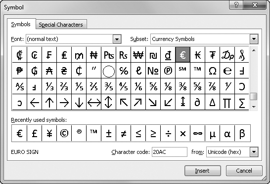
If you ever want to use characters in Excel that are not on your standard computer keyboard, you’re in luck. Clicking the Insert tab on the ribbon and then clicking the Symbol button gives you access to the complete character set for every installed font on your computer. Figure 6-11 shows the Symbol dialog box.
On the Symbols tab, select the font from the Font drop-down list; the entire character set appears. You can jump to specific areas in the character set by using the Subset drop-down list, which also indicates the area of the character set you are viewing if you are using the scroll bar to browse through the available characters. The Character Code box displays the code for the selected character. You can also highlight a character in the display area by typing the character’s code number. You can select decimal or hexadecimal ASCII character encoding or Unicode by using the From drop-down list. If you choose Unicode, you can select from a number of additional character subsets in the Subset drop-down list. The Special Characters tab in the Symbol dialog box gives you quick access to a number of commonly used characters, such as the em dash, the ellipsis, and the trademark and copyright symbols.
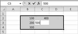
To make a number of entries in a range of adjacent cells, first select all of them. Then just begin typing entries, as shown in Figure 6-12. Each time you press Enter, the active cell moves to the next cell in the range, and the range remains selected. When you reach the edge of the range and press Enter, the active cell jumps to the beginning of the next column or row. You can continue making entries this way until you fill the entire range.
You can correct simple errors as you type by pressing Backspace. However, to make changes to entries you have already locked in, you first need to enter Edit mode. (The mode indicator at the lower-left corner of the status bar has to change from Ready to Edit.) To enter Edit mode, do one of the following:
Double-click the cell and position the insertion point at the location of the error.
Select the cell and press F2. Use the arrow keys to position the insertion point within the cell.
To select contiguous characters within a cell, place the insertion point just before or just after the characters you want to replace, and press Shift+Left Arrow or Shift+Right Arrow to extend your selection.
Note
If you don’t want to take your hands off the keyboard to move from one end of a cell entry to the other, press Home or End while in Edit mode. To move through an entry one “word” at a time, press Ctrl+Left Arrow or Ctrl+Right Arrow.
If you need to erase the entire contents of the active cell, press Delete, or press Backspace and then Enter. If you press Backspace accidentally, click the Cancel button or press Esc to restore the contents of the cell before pressing Enter. You can also erase the entire contents of a cell by selecting the cell and typing new contents to replace the old. To revert to the original entry, press Esc before you press Enter.


You can always click the Undo button in the Quick Access Toolbar; alternatively, press Ctrl+Z. The Undo button remembers the last 100 actions you performed. If you press Ctrl+Z repeatedly, each of the last 100 actions is undone, one after the other, in reverse order. You can also click the small arrow next to the Undo button to display a list of remembered actions. Drag the mouse to select one or more actions, as shown in Figure 6-13. After you release the mouse, all the selected actions are undone. The Redo button works the same way; you can quickly redo what you have just undone, if necessary.
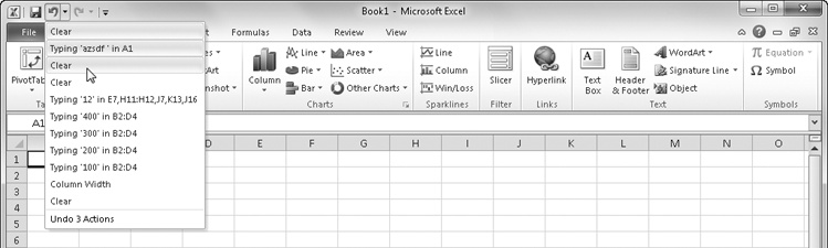
Figure 6-13. Click the small arrow next to the Undo button to select any number of the last 16 actions to undo at once.
Note
You can’t undo individual actions in the middle of the Undo list. If you select an action, all actions up to and including that action are undone.
Floating Option Buttons
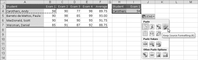
There are several different types of “floating” option buttons that appear as you work in Excel. These are provided to give you instant access to commands and actions that are relevant to the current task. Many editing actions trigger the display of an option button. For example, copying and pasting cells causes the Paste Options button to appear adjacent to the last cell edited. If you click the button, a menu offers retroactive editing options:
Floating option buttons appear in many situations, so you will hear about them in other places in this book. For examples, see Tracing Errors on page 270, Pasting Selectively Using Paste Special on page 203, and Entering a Series of Dates on page 568.