Because SUM is such a commonly used function, Excel provides the Sum button on the Home tab on the ribbon, as well as the AutoSum button on the Formulas tab. In addition to SUM, these buttons include a menu of other commonly used functions. If you select a cell and click the Sum button, Excel creates a SUM formula and guesses which cells you want to total. To enter SUM formulas in a range of cells, select the cells before clicking Sum.

The SUMIF function is similar to SUM, but it first tests each cell using a specified conditional test before adding it to the total. This function takes the arguments (range, criteria, sum_range). The range argument specifies the range you want to test, the criteria argument specifies the conditional test to be performed on each cell in the range, and the sum_range argument specifies the cells to be totaled. For example, if you have a worksheet with a column of month names defined using the range name Months and an adjacent column of numbers named Sales, use the formula =SUMIF(Months, “June”, Sales) to return the value in the Sales cell that is adjacent to the label June. Alternatively, you can use a conditional test formula such as =SUMIF(Sales, “>=999”, Sales) to return the total of all sales figures that are more than $999.

The SUMIFS function does similar work to that of the SUMIF function, except you can specify up to 127 different conditional ranges, each with their own criteria. Note that in this function, the sum_range argument is in the first position instead of the third position: (sum_range, criteria_range1, criteria1, criteria_range2, criteria2, …). The sum range and each criteria range must all be the same size and shape. Using a similar example to the one we used for the SUMIF function, suppose we also created defined names for cell ranges Months, Totals, Product1, Product2, and so on. The formula =SUMIFS(Totals, Product3, “<=124”, Months, “June”) returns the total sales for the month of June when sales of Product3 were less than or equal to $124.

Similarly, COUNTIF counts the cells that match specified criteria and takes the arguments (range, criteria). Using the same example, you can find the number of months in which total sales fell to less than $600 by using a conditional test, as in the formula =COUNTIF(Totals, “<600”).

The PRODUCT function multiplies all its arguments and can take as many as 255 arguments that are text or logical values; the function ignores blank cells.

You can use the SUMPRODUCT function to multiply the value in each cell in one range by the corresponding cell in another range of equal size and then add the results. You can include up to 255 arrays as arguments, but each array must have the same dimensions. (Non-numeric entries are treated as zero.) For example, the following formulas are essentially the same:

=SUMPRODUCT(A1:A4, B1:B4)
{=SUM(A1:A4*B1:B4)}

The only difference between them is that you must enter the SUM formula as an array by pressing Ctrl+Shift+Enter.

The MOD function returns the remainder of a division operation (modulus). It takes the arguments (number, divisor). The result of the MOD function is the remainder produced when number is divided by divisor. For example, the function =MOD(9, 4) returns 1, the remainder that results from dividing 9 by 4.

The COMBIN function determines the number of possible combinations, or groups, that can be taken from a pool of items. It takes the arguments (number, number_chosen), where number is the total number of items in the pool and number_chosen is the number of items you want to group in each combination. For example, to determine how many different 11-player football teams you can create from a pool of 17 players, type the formula =COMBIN(17, 11). The result indicates that you could create 12,376 teams.

The RAND function generates a random number between 0 and 1. It’s one of the few Excel functions that doesn’t take an argument, but you must still type a pair of parentheses after the function name. The result of a RAND function changes each time you recalculate your worksheet. This is called a volatile function. If you use automatic recalculation, the value of the RAND function changes each time you make a worksheet entry.

The RANDBETWEEN function provides more control than RAND. With RANDBETWEEN, you can specify a range of numbers within which to generate random integer values. The arguments (bottom, top) represent the smallest and largest integers that the function should use. The values for these arguments are inclusive. For example, the formula =RANDBETWEEN(123, 456) can return any integer from 123 up to and including 456.

A MOD Example

Here’s a practical use of the MOD function that you can ponder:

1. Select a range of cells such as B5:F16, click Conditional Formatting on the Home tab on the ribbon, and then click New Rule.

2. Select the Use A Formula To Determine Which Cells To Format option in the Select A Rule Type list.

3. In the text box, type the formula =MOD(ROW(), 2)=0.

4. Click the Format button, and select a color on the Fill tab to create a format that applies the selected color to every other row. Note that if you select a single cell in an odd-numbered row before creating this formatting formula, nothing seems to happen, but if you copy or apply the format to other rows, you’ll see the result. Click OK.

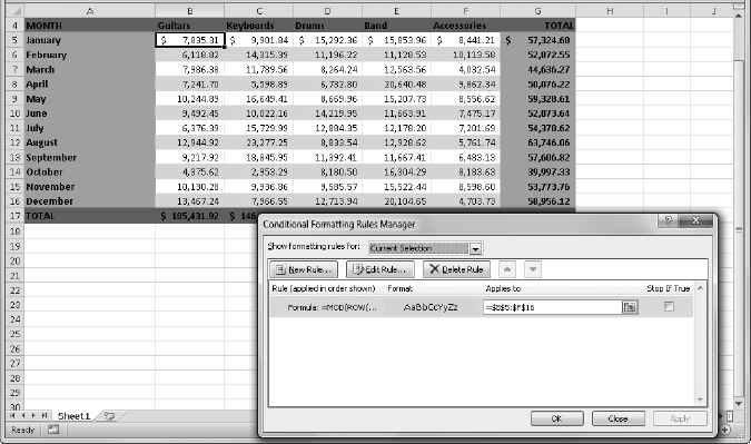
We clicked the Conditional Formatting button and clicked Manage Rules to display the dialog box shown in the preceding figure. The MOD formula identifies the current row number using the ROW function, divides it by 2, and if there is a remainder (indicating an odd-numbered row), returns FALSE because the formula also contains the conditional test =0. If MOD returns anything but 0 as a remainder, the condition tests FALSE. Therefore, Excel applies formatting only when the formula returns TRUE (in even-numbered rows). For more information about conditional formatting, see Formatting Conditionally on page 309. You can also achieve similar results (with additional functionality) by converting the cell range into a table and using the table formatting features. For more information, see Chapter 22.

The ROUND function rounds a value to a specified number of decimal places. Digits to the right of the decimal point that are less than 5 are rounded down, and digits greater than or equal to 5 are rounded up. It takes the arguments (number, num_digits). If num_digits is a positive number, then number is rounded to the specified number of decimal points; if num_digits is negative, the function rounds to the left of the decimal point; if num_digits is 0, the function rounds to the nearest integer. For example, the formula =ROUND(123.4567, –2) returns 100, and the formula =ROUND(123.4567, 3) returns 123.457. The ROUNDDOWN and ROUNDUP functions take the same form as ROUND. As their names imply, they always round down or up, respectively.

Caution

Don’t confuse the rounding functions with rounded number formats, such as the one applied when you click the Accounting Number Format button on the Home tab on the ribbon. When you format the contents of a cell to a specified number of decimal places, you change only the display of the number in the cell; you don’t change the cell’s value. When performing calculations, Excel always uses the underlying value, not the displayed value. Conversely, the rounding functions permanently change the underlying values.

The EVEN function rounds a number up to the nearest even integer. The ODD function rounds a number up to the nearest odd integer. Negative numbers are correspondingly rounded down. For example, the formula =EVEN(22.4) returns 24, and the formula =ODD(–4) returns –5.

The FLOOR function rounds a number down to its nearest given multiple, and the CEILING function rounds a number up to its nearest given multiple. These functions take the arguments (number, multiple). For example, the formula =FLOOR(23.4, 0.5) returns 23, and the formula =CEILING(5, 1.5) returns 6, the nearest multiple of 1.5. The FLOOR.PRECISE and CEILING.PRECISE functions (both new in Excel 2010) round numbers down or up to the nearest integer or multiple of significance. Both take the arguments (number, significance). For example, the formula =FLOOR.PRECISE(23.4, 4) returns 20, which is the nearest integer below 23.4 that is a multiple of 4. Most of the time, you see no difference in results between the regular and precise versions of these functions, unless your arguments are negative numbers. The precise versions always round up, regardless of the number’s sign.

The INT function rounds numbers down to the nearest integer. For example, the formulas

=INT(100.01)
=INT(100.99999999)

both return the value 100, even though the number 100.99999999 is essentially equal to 101. When a number is negative, INT also rounds that number down to the next integer. If each of the numbers in these examples were negative, the resulting value would be –101.

The TRUNC function truncates everything to the right of the decimal point in a number, regardless of its sign. It takes the arguments (number, num_digits). If num_digits isn’t specified, it’s set to 0. Otherwise, TRUNC truncates everything after the specified number of digits to the right of the decimal point. For example, the formula =TRUNC(13.978) returns the value 13; the formula =TRUNC(13.978, 1) returns the value 13.9.