
The Goal Seek command is handy for problems that involve an exact target value that depends on a single unknown value. For problems that are more complex, you should use the Solver add-in. The Solver can handle problems that involve many variable cells and can help you find combinations of variables that maximize or minimize a target cell. It also specifies one or more constraints—conditions that must be met for the solution to be valid.
Note
The Solver is an add-in. If the Solver button does not appear on the Data tab on the ribbon, click the File tab, Options, Add-Ins category, and then click the Go button. Select the Solver Add-In check box, and then click OK to install it.
As an example of the kind of problem that the Solver can tackle, imagine you are planning an advertising campaign for a new product. Your total budget for print advertising is $12,000,000; you want to expose your ads at least 800 million times to potential readers; and you’ve decided to place ads in six publications—we’ll call them Pub1 through Pub6. Each publication reaches a different number of readers and charges a different rate per page. Your job is to reach the readership target at the lowest possible cost with the following additional constraints:
Figure 18-23 shows one way to lay out the problem.

Figure 18-23. You can use the Solver to determine how many advertisements to place in each publication to meet your objectives at the lowest possible cost.
Note
This section merely introduces the Solver. A complete treatment of this powerful tool is beyond the scope of this book. For more details, including an explanation of the Solver error messages, see the Help system. For background material about optimization, we recommend Financial Models Using Simulation and Optimization II: Investment by Wayne L. Winston (Palisade Corporation, 2001).
You might be able to work out this problem yourself by substituting many alternatives for the values currently in D2:D7, keeping your eye on the constraints, and noting the impact of your changes on the total expenditure figure in E8. In fact, that’s what the Solver does for you—but it does it more rapidly, and it uses some analytic techniques to home in on the optimal solution without having to try every conceivable alternative.
Click the Solver button on the Data tab to display the dialog box shown in Figure 18-24. To complete this dialog box, you must give the Solver three sets of information: your objective (minimizing total expenditure); your variable cells (the number of advertisements you will place in each publication); and your constraints (the conditions summarized at the bottom of the worksheet in Figure 18-23).

In the Set Objective box, you indicate the goal that you want Solver to achieve. In this example, you want to minimize your total cost—the value in cell E8—so you specify your objective by typing E8 in the Set Objective box (or by clicking the cell). In this example, because you want the Solver to set your objective to its lowest possible value, also select the Min option.
Note
It’s a good idea to name all the important cells of your model before you put the Solver to work. If you don’t name the cells, the Solver constructs names to use on its reports based on the nearest column-heading and row-heading text, but these constructed names don’t appear in the Solver dialog boxes. For more information, see Naming Cells and Cell Ranges on page 483.
You don’t have to specify an objective. If you leave the Set Objective box blank, click Options, and then select the Show Iteration Results check box, you can use the Solver to step through some or all the combinations of variable cells that meet your constraints. You then receive an answer that solves the constraints but isn’t necessarily the optimal solution.
Note
For more information about the Show Iteration Results option, see Viewing Iteration Results on page 663.
The next step is to tell the Solver which cells to change. In our example, the cells whose values can be adjusted are those that specify the number of advertisements to be placed in each publication, or cells D2:D7. You can specify up to 200 variable cells, and they can be nonadjacent (unlike our example). When you enter nonadjacent cell references or named ranges, separate them with commas.
The last step, specifying constraints, is optional. To specify a constraint, click Add in the Solver Parameters dialog box, and complete the Add Constraint dialog box. Figure 18-25 shows how you express the constraint that total advertising expenditures (the value in cell E8 in the model) must be less than or equal to the total budget (the value in cell G11).

Figure 18-26 shows how the Solver Parameters dialog box looks after we have specified all our constraints.
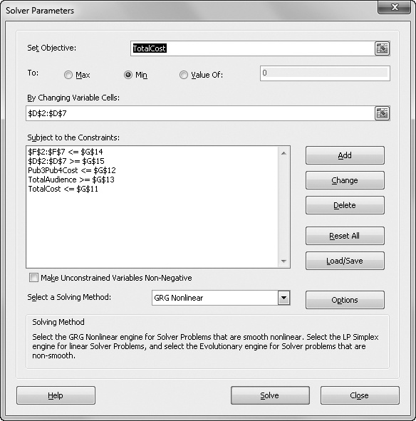
Figure 18-26. The Solver lists the constraints and uses defined cell and range names whenever possible.
Notice that two of the constraints have range references on the left side of the comparison operator. The expression $D$2:$D$7>=$G$15 stipulates that the value of each cell in D2:D7 must be 6 or greater, and the expression $F$2:$F$7<=$G$14 stipulates that the value of each cell in F2:F7 must be no greater than 33.30 percent. Each of these expressions is a shortcut way of stating six separate constraints. If you use this kind of shortcut, the constraint value on the right side of the comparison operator must be a single cell reference, a range of the same dimensions as the range on the left side, or a constant value.
After completing the Solver Parameters dialog box, click Solve. In the advertisement campaign example, the Solver succeeds in finding an optimal value for the objective cell while meeting all the constraints and displays the dialog box shown in Figure 18-27. The values displayed on your worksheet at that time result in the optimal solution. You can leave these values in the worksheet by selecting the Keep Solver Solution option and clicking OK, or you can restore the original values by selecting the Restore Original Values option and clicking OK (or by clicking Cancel). You also have the option of assigning the solution values to a named scenario.
Notice that in Figure 18-27, the Solver arrived at 53.3 for the number of ads placed in Pub4. Unfortunately, because it’s not possible to run three-tenths of an advertisement, the solution isn’t practical.

To stipulate that your ad-placement variables be restricted to whole numbers, start the Solver, and click the Add button in the Solver Parameters dialog box. In the Add Constraint dialog box, you select the cell reference that holds your ad placement numbers—D2:D7. Click the list in the middle of the dialog box, and select int. The Solver inserts the word integer in the Constraint box, as shown in Figure 18-28. Click OK to return to the Solver Parameters dialog box.

Note that when Excel converts numbers to integers, the program effectively rounds down; the decimal portion of the number is truncated. The integer solution shows that by placing 53 ads in Pub4, you can buy an additional ad in Pub5. For a very small increase in budget, you can reach an additional two million readers.
In the Solver Parameters dialog box, the Select A Solving Method drop-down list offers three options: GRG Nonlinear (the default), Simplex LP, and Evolutionary. Simply put, the differences are:
GRG Nonlinear The default solving method is optimized for “smooth nonlinear” problems involving points along a curved (but smooth) line.
Simplex LP This method works best for linear problems that can be defined as points along a straight line.
Evolutionary This option works best when your model involves “non-smooth”, or random, discontinuous elements that would not plot along either a straight or curved line.
Click the Options button in the Solver Parameters dialog box to display the Options dialog box shown in Figure 18-29, which contains many additional settings. It’s best to leave the options on the GRG Nonlinear and Evolutionary tabs at their default settings—unless you understand linear optimization techniques. The following options on the All Methods tab bear some explanation:
The Constraint Precision setting determines how closely you want values in the constraint cells to match your constraints. The closer this setting is to the value 1, the lower the precision is. If you specify a setting that is less than the default 0.000001, it results in a longer solution time.
The Max Time and Iterations boxes tell the Solver, in effect, how hard to work on the solution. If the Solver reaches either the time limit or the number of iterations limit before finding a solution, calculation stops, and Excel asks you whether you want to continue. The default settings are usually sufficient for solving most problems, but if you don’t reach a solution with these settings, you can try adjusting them.
The Integer Optimality (%) setting represents a percentage of error allowed for the solution of integer-only constraints.

Note
This section only scratches the surface of optimization theory. There is extensive reading available on the subject. For evidence, type “nonlinear optimization” into your browser’s Search box and scan the results. You can click the Help button in the Solver Parameters dialog box to display the Excel Help topic on the Solver, where you will find a link at the bottom of the page to the Web site of Frontline Systems (the developers of the Solver) for additional help, resources, and even upgrades for the Solver.
A linear optimization problem is one in which the value of the target cell is a linear function of each variable cell; that is, if you plot X Y (scatter) charts of the target cell’s value against all meaningful values of each variable cell, your charts are straight lines. If some of your plots produce curves instead of straight lines, the problem is nonlinear.
In the Solver Parameters dialog box, you can use the Simplex LP option in the Select A Solving Method drop-down list only for what-if models in which all the relationships are linear. Models that use simple addition and subtraction and worksheet functions such as SUM are linear in nature. However, most models are nonlinear. They are generated by multiplying changing cells by other changing cells, by using exponentiation or growth factors, or by using nonlinear worksheet functions, such as PMT.
Linear problems can be solved more quickly by using the Simplex LP option. However, if you select this option for a nonlinear problem and then try to solve the problem, the Solver Results dialog box displays an error message. If you are not sure about the nature of your model, it’s best not to use this option.
If you’re interested in exploring many combinations of your variable cells, rather than only the combination that produces the optimal result, click Options in the Solver Parameters dialog box and select the Show Iteration Results check box. When you do, the Show Trial Solution dialog box appears after each iteration, which allows you to save the scenario and then either stop the trial or continue with the next iteration.
Be aware that if you use Show Iteration Results, the Solver pauses for solutions that do not meet all your constraints, as well as for suboptimal solutions that do.
If you save a workbook after using the Solver, Excel saves all the values you typed in the Solver dialog boxes along with your worksheet data. You do not need to retype the parameters of the problem if you want to continue working with it during a later Excel session.
Each worksheet in a workbook can store one set of Solver parameter values. To store more than one set of Solver parameters with a given worksheet, you must use the Save Model option. To use this option, follow these steps:
Click the Solver button on the Data tab.
Click the Load/Save button. Excel prompts you for a cell or range in which to store the Solver parameters on the worksheet.
Specify a blank cell by clicking it or typing its reference, and then click Save. The Solver pastes the model beginning at the indicated cell and inserts formulas in as many of the cells below it as necessary. (Be sure that the cells below the indicated cell do not contain data.)
To reuse the saved parameters, click Load/Save in the Solver Parameters dialog box, specify the range in which you stored the Solver parameters, as shown in Figure 18-30, and then click Load.

You’ll find it easiest to save and reuse Solver parameters if you assign a name to each save-model range immediately after you use the Save Model option. You can then specify that name when you use the Load Model option.
Note
For more information about naming, see Naming Cells and Cell Ranges on page 483.
An even better way to save your Solver parameters is to save them as named scenarios using the Scenario Manager. As you might have noticed, the Solver Results dialog box includes a Save Scenario button (refer to Figure 18-27). Click this button to assign a scenario name to the current values of your variable cells. This option provides an excellent way to explore and perform further what-if analysis on a variety of possible outcomes.
Note
For more information about scenarios, see Using the Scenario Manager on page 641.
In addition to inserting optimal values in your problem’s variable cells, the Solver can summarize its results in three reports: Sensitivity, Answer, and Limits. To generate one or more reports, select the names of the reports in the Solver Results dialog box. Select the reports you want, and then click OK. Each report is saved on a separate worksheet in the current workbook.
The Sensitivity report provides information about how sensitive your target cell is to changes in your constraints. This report has two sections: one for your variable cells and one for your constraints. The right column in each section provides the sensitivity information.
Each changing cell and constraint cell appears in a separate row. The Changing Cell area includes a Reduced Gradient value that indicates how the target cell would be affected by a one-unit increase in the corresponding changing cell. Similarly, the Lagrange Multiplier column in the Constraints area indicates how the target cell would be affected by a one-unit increase in the corresponding constraint value.
The Answer report lists the target cell, the variable cells, and the constraints. This report also includes information about the status of and slack value for each constraint. The status can be Binding, Not Binding, or Not Satisfied. The slack value is the difference between the solution value of the constraint cells and the number that appears on the right side of the constraint formula. A binding constraint is one for which the slack value is 0. A nonbinding constraint is a constraint that was satisfied with a nonzero slack value.
The Limits report tells you how much you can increase or decrease the values of your variable cells without breaking the constraints of your problem. For each variable cell, this report lists the optimal value as well as the lowest and highest values that you can use without violating constraints.
TROUBLESHOOTING
The Solver can’t solve my problem.
The Solver is powerful but not miraculous. It might not be able to solve every problem you give it. This is not always because the problem cannot be solved; sometimes it is because you need to provide better starting parameters. If the Solver can’t find the optimal solution to your problem, it presents an unsuccessful completion message in the Solver Results dialog box. The most common unsuccessful completion messages are the following:
Solver could not find a feasible solution The Solver is unable to find a solution that satisfies all your constraints. This can happen if the constraints are logically conflicting or if not all the constraints can be satisfied (for example, if you insist that your advertising campaign reach 800 million readers on a $1 million budget). In some cases, the Solver also returns this message if the starting values of your variable cells are too far from their optimal values. If you think your constraints are logically consistent and your problem is solvable, try changing your starting values and rerunning the Solver.
The maximum iteration limit was reached; continue anyway? To avoid tying up your computer indefinitely with an unsolvable problem, the Solver is designed to pause and present this message after it has performed its default number of iterations without arriving at a solution. If you see this message, you can resume the search for a solution by clicking Continue, or you can quit by clicking Stop. If you click Continue, the Solver begins solving again and does not stop until it finds a solution, gives up, or reaches its maximum time limit. If your problems frequently exceed the iteration limit, you can increase the default iteration setting by clicking the Solver button on the Data tab, clicking the Options button, and typing a new value in the Iterations box.
The maximum time limit was reached; continue anyway? This message is similar to the iteration-limit message. The Solver is designed to pause after a default time period has elapsed. You can increase this default by choosing the Solver command, clicking Options, and modifying the Max Time value.