
The formatting features in Excel 2010 control the display characteristics of numbers and text. It is important to keep in mind the difference between underlying and displayed worksheet values. Formats do not affect the underlying numeric or text values in cells. For example, if you type a number with six decimal places in a cell that is formatted with two decimal places, Excel displays the number with only two decimal places. However, the underlying value isn’t changed, and Excel uses the underlying value in calculations.
Note
When you copy a cell or range of cells, you copy both its contents and its formatting. If you then paste this information into another cell or range, the formatting of the source cells normally replaces any existing formatting. For more information about copying and pasting, see Chapter 8.
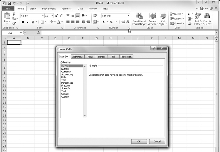
Most of your formatting needs should be quickly and easily fulfilled using buttons and controls located on the Home tab on the ribbon, but for more options, you can employ the Format Cells dialog box. To display the Format Cells dialog box, press Ctrl+1. Alternatively, click one of the dialog box launchers adjacent to the titles of the Font, Alignment, and Number groups on the Home tab. Clicking a dialog box launcher also activates the corresponding tab. Figure 9-32 shows the Format Cells dialog box.
Throughout the following sections we’ll discuss formatting options available directly on the ribbon, but we’ll go into more depth by employing the Format Cells dialog box.
If you select a cell and apply formats, the entire contents of the cell receive the formats. However, you can also apply formatting to individual text characters within cells (but not numeric values or formulas). Select individual characters or words inside a cell, and apply the attributes you want. When you are finished, press Enter to see the results, an example of which is shown in Figure 9-33.
Note
For more examples of formatting individual characters, see Using Fonts on page 351.

You can include special formatting characters—such as dollar signs, percent signs, commas, or fractions—to format numbers as you type them. When you type numeric-entry characters that represent a format Excel recognizes, Excel applies that format to the cell on the fly. The following list describes some of the more common special formatting characters:
If you type $45.00 in a cell, Excel interprets your entry as the value 45 formatted as currency with two decimal places. Only the value 45 appears in the formula bar after you press Enter, but the formatted value, $45.00, appears in the cell.
If you type 1 3/8 (with a single space between 1 and 3), 1 3/8 appears in the cell and 1.375 appears in the formula bar. However, if you type 3/8, then 8-Mar appears in the cell, because date formats take precedence over fraction formats. Assuming you make the entry in the year 2010, then 3/8/2010 appears in the formula bar. To display 3/8 in the cell as a fraction so that 0.375 appears in the formula bar, you must type 0 3/8 (with a space between 0 and 3). For information about typing dates and a complete listing of date and time formats, see Entering Dates and Times on page 566.
If you type 23% in a cell, Excel applies the no-decimal percentage format to the cell, and 23% appears in the formula bar. Nevertheless, Excel uses the 0.23 decimal value for calculations.
If you type 123,456 in a cell, Excel applies the comma format without decimal places. If you type 123,456.00, Excel formats the cell with the comma format including two decimal places.
Note
Leading zeros are almost always dropped, unless you create or use a format specifically designed to preserve them. For example, when you type 0123 in a cell, Excel displays the value 123, dropping the leading zero. Excel provides custom formats for a couple of commonly needed leading-zero applications, namely ZIP codes and social security numbers, on the Number tab, Special category of the Format Cells dialog box. For more information, see Using the Special Formats on page 332. For information about creating your own formats, see Creating Custom Number Formats on page 333.
The General format is the default format for all cells. Although it is not just a number format, it is nonetheless always the first number format category listed. Unless you specifically change the format of a cell, Excel displays any text or numbers you type in the General format. Except in the cases listed next, the General format displays exactly what you type. For example, if you type 123.45, the cell displays 123.45. Here are the four exceptions:
The General format abbreviates numbers too long to display in a cell. For example, if you type 12345678901234 (an integer) into a standard-width cell, Excel displays 1.23457E+13.
Long decimal values are also rounded or displayed in scientific notation. Thus, if you type 123456.7812345 in a standard-width cell, the General format displays 123456.8. The actual typed values are preserved and used in all calculations, regardless of the display format.
The General format does not display trailing zeros. For example, if you type 123.0, Excel displays 123.
A decimal fraction typed without a number to the left of the decimal point is displayed with a zero. For example, if you type .123, Excel displays 0.123.
The second option in the drop-down list displayed in the Number group on the Home tab is called, helpfully, Number. When you use the drop-down list, selecting Number applies a default number format, with two decimal places and comma separators. For example, if you apply the Number format with a cell selected containing 1234.556, the cell displays the number as 1,234.56. Excel rounds the decimal value to two places in the process, which does not change the actual value in the cell, just the displayed value.
Note

The Comma Style button in the Number group on the Home tab applies the same format as does the Number format in the drop-down list.
In the Format Cells dialog box, the Number category contains additional options, letting you display numbers in integer, fixed-decimal, and punctuated formats, as shown in Figure 9-34. It is essentially the General format with additional control over displayed decimal places, thousand separators, and negative numbers. You can use this category to format any numbers that do not fall into any of the other categories.
Follow these guidelines when using the Number category:
Select the number of decimal places to display (0 to 30) by typing or scrolling to the value in the Decimal Places box.
Select the Use 1000 Separator (,) check box to add commas between hundreds and thousands, and so on.
Select an example in the Negative Numbers list to display negative numbers preceded by a minus sign, in red, in parentheses, or in both red and parentheses.
Note
When formatting numbers, always select a cell containing a number before opening the Format Cells dialog box so that you can see the actual results in the Sample area.

The quickest way to apply currency formatting is by clicking Currency in the Number drop-down list in the Number group on the Home tab, as shown in Figure 9-35. The Currency format is similar to the Number format that precedes it in the drop-down list, except it also includes the default currency symbol for your locale. Notice that most of the commands listed here display little previews showing you what the contents of the active cell will look like if you click that command.
Note
Despite the button’s appearance, clicking the $ button on the Home tab actually applies a two-decimal Accounting format, which is similar to, but a little different from, the Currency format. We’ll discuss Accounting formats in the next section.
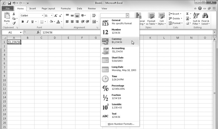
Figure 9-35. The contents of the selected cell are previewed below each command in the Number drop-down list.
For additional currency formatting options, select the Currency category in the Format Cells dialog box, which offers a similar set of options as the Number category (refer to Figure 9-34) but adds a drop-down list of worldwide currency symbols. Besides clicking the dialog box launcher in the Number group on the Home tab to display the Format Cells dialog box, you can also select the More Number Formats command at the bottom of the Number drop-down list shown in Figure 9-35.
Using the Decimal Buttons
You can change the number of displayed decimal places in any selected cell or range at any time using two buttons—Increase Decimal and Decrease Decimal—in the Number group on the Home tab:
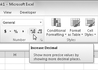
The Increase Decimal button displays an arrow pointing to the left, and the Decrease Decimal button displays an arrow pointing to the right, which might seem backward to those of us in the left-to-right/smaller-to-larger world of Western culture, but of course these buttons address what happens only on the right side of the decimal point. Each click adds or subtracts one decimal place from the displayed value. Interestingly, although you can specify up to 30 decimal places using the Format Cells dialog box, you can increase the number of decimal places to a maximum of 127, one click at a time, using the Increase Decimal button.
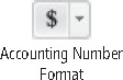
The most-often-used Accounting format is directly available on the Home tab on the ribbon, using the Accounting Number Format button in the Number group. Clicking this button applies a standard two-decimal-place format with comma separators and currency symbols to the selected cells. Clicking the arrow button adjacent to the Accounting Number Format button displays a menu providing access to a few additional currency symbols, as shown in Figure 9-36.

Figure 9-36. The $ button applies a standard Accounting format and offers a few optional currency symbols.
The Accounting formats address the needs of accounting professionals, but they benefit the rest of us as well. When you use one of these formats with the Single Accounting or Double Accounting font formats (to add underlines to your numbers), you can easily create profit and loss (P&L) statements, balance sheets, and other schedules that conform to generally accepted accounting principles (GAAP). The Accounting formats correspond roughly to the Currency format in appearance—you can display numbers with or without your choice of currency symbols and specify the number of decimal places. However, the two formats have some distinct differences. The rules governing the Accounting formats are as follows:
The Accounting format displays every currency symbol flush with the left side of the cell and displays numbers flush with the right side, as shown in Figure 9-36. The result is that all the currency symbols in the same column are vertically aligned, which looks much cleaner than Currency formats.
In the Accounting format, negative values are always displayed in parentheses and always in black—displaying numbers in red is not an option.
The Accounting format includes a space equivalent to the width of a parenthesis on the right side of the cell so that numbers line up evenly in columns of mixed positive and negative values.
The Accounting format displays zero values as dashes. The spacing of the dashes depends on whether you select decimal places. If you include two decimal places, the dashes line up under the decimal point.
Finally, the Accounting format is the only built-in format that includes formatting criteria for text. It includes spaces equivalent to the width of a parenthesis on each side of text so that it too lines up evenly with the numbers in a column.
Typically, when creating a GAAP-friendly worksheet of currency values, you would use currency symbols only in the top row and in the totals row at the bottom of each column of numbers. This makes good sense because using dollar signs with every number would make for a much busier table. The middle of the table is then formatted using a compatible format without currency symbols, as shown in Figure 9-37.

Figure 9-37. It is standard practice to use currency symbols only in the top and bottom rows of a table.
Luckily, Excel makes it easy for you to format this way by using buttons in the Number group on the Home tab. Despite seemingly incompatible button names, both the Accounting Number Format button and the Comma Style button apply Accounting formats adhering to the rules described earlier. So, to format the numeric entries in the table shown in Figure 9-37, select the first and last rows, click the Accounting Number Format button, then select all the cells in between, and click the Comma Style button. (We then selected all the numeric cells in the table and clicked the Decrease Decimal button twice to hide all the decimal values.)
Note
For information about font formats, see Using Fonts on page 351. For information about tables, see Formatting Tables on page 292.
Not surprisingly, using the Percentage format displays numbers as percentages. The decimal point of the formatted number, in effect, moves two places to the right, and a percent sign appears at the end of the number. For example, if you choose a percentage format without decimal places, the entry 0.1234 is displayed as 12%; if you select two decimal places, the entry 0.1234 is displayed as 12.34%. Remember that you can always adjust the number of displayed decimal places using the Increase Decimal and Decrease Decimal buttons.

An interesting (and helpful) quirk about percentage formats is that they behave differently depending on whether you type a number and then apply the format or type a number in a previously formatted cell. For example, Figure 9-38 shows two cells formatted as percentages. We typed the same number—22.33—in each cell, but only cell A1 was previously formatted with the Percentage format; we clicked the Percent Style button after typing the value in cell A2.
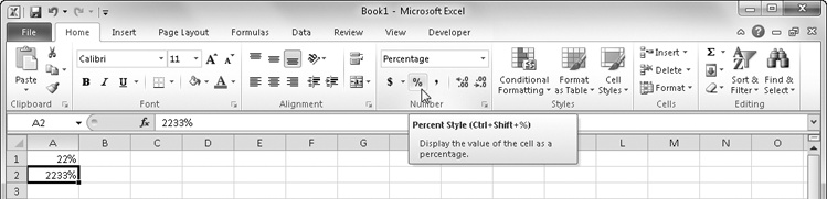
Figure 9-38. When using percentages, it makes a difference whether you format before or after typing values.
As you can see, it makes a world of difference which way you do this. So, why is this behavior helpful? For example, if a worksheet contains a displayed value of 12% and you need to change it to 13%, typing 13 in the cell would seem to make sense, even though this is technically wrong. It is not particularly intuitive to type .13 (including the leading decimal point). Usability studies show that most people would type 13 in this situation, which would logically result in a displayed value of 1300% (if not for the quirky behavior), so Excel assumes that you want to display 13%. If you apply the Percentage format to a range of cells that already contain values (or formulas that result in values), check all the cells afterward to make sure you get the intended results.
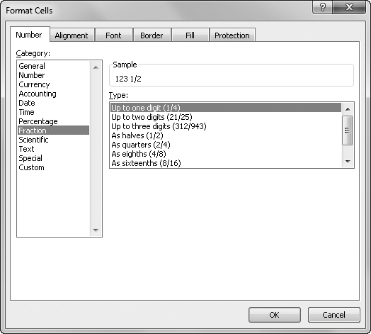
The formats in the Fraction category in the Format Cells dialog box, shown in Figure 9-39, display fractional numbers as actual fractions rather than as decimal values. As with all number formats, the underlying value does not change despite the displayed value of the fraction.
You can generate some wild, nonstandard fractions unless you apply constraints using options in the Format Cells dialog box. Here is how Excel applies different fraction formats:
The Up To One Digit (single-digit) fraction format displays 123.456 as 123 1/2, rounding the display to the nearest value that can be represented as a single-digit fraction.
The Up To Two Digits (double-digit) fraction format uses the additional precision allowed by the format and displays 123.456 as 123 26/57.
The Up To Three Digits (triple-digit) fraction format displays 123.456 as the even more precise 123 57/125.
The remaining six fraction formats specify the exact denominator you want by rounding to the nearest equivalent; for example, displaying 123.456 using the As Sixteenths format, or 123 7/16.
Note
You can also apply fraction formatting on the fly by typing fractional values in a specific way. Type a number (or a zero), type a space, and then type the fraction, as in 123 1/2. For more details, see Formatting as You Type on page 322.
The Scientific format displays numbers in exponential notation. For example, a two-decimal Scientific format (the default) displays the number 98765432198 as 9.88E+10 in a standard-width cell. The number 9.88E+10 is 9.88 times 10 to the 10th power. The symbol E stands for exponent, a synonym here for 10 to the nth power. The expression “10 to the 10th power” means 10 times itself 10 times, or 10,000,000,000. Multiplying this value by 9.88 gives you 98,800,000,000, an approximation of 98,765,432,198. Increasing the number of decimal places (the only option available for this format) increases the precision and will likely require a wider cell to accommodate the displayed value.
You can also use the Scientific format to display very small numbers. For example, in a standard-width cell this format displays 0.000000009 as 9.00E–09, which equates to 9 times 10 to the negative 9th power. The expression “10 to the negative 9th power” means 1 divided by 10 to the 9th power, 1 divided by 10 nine times, or 0.000000001. Multiplying this number by nine results in our original number, 0.000000009.
Applying the Text format to a cell indicates that the entry in the cell is to be treated as text, even if it’s a number. For example, a numeric value is ordinarily right-aligned in its cell. If you apply the Text format to the cell, however, the value is left-aligned as if it were a text entry. For all practical purposes, a numeric constant formatted as text is still considered a number because Excel is capable of recognizing its numeric value anyway.
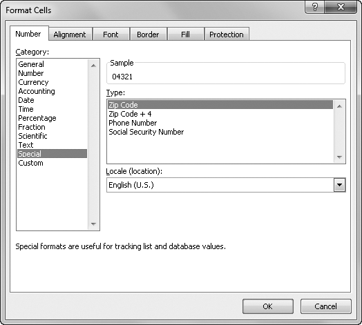
The four Special formats shown in Figure 9-40 are a result of many requests from users. These generally noncalculated numbers include two ZIP code formats, a phone number format (complete with the area code in parentheses), and a Social Security number format. Using each of these Special formats, you can quickly type numbers without having to type the punctuation characters.
The following are guidelines for using the Special formats:
Zip Code and Zip+4 Leading zeros are retained to correctly display the code, as in 04321. In most other number formats, if you type 04321, Excel drops the zero and displays 4321.
Phone Number Excel applies parentheses around the area code and dashes between the digits, making it much easier to type many numbers at the same time because you don’t have to move your hand from the keypad. Furthermore, the numbers you type remain numbers instead of becoming text entries, which they would be if you typed parentheses or dashes in the cell.
Social Security Number Excel places dashes after the third and fifth numbers. For example, if you type 123456789, Excel displays 123-45-6789.
Locale This drop-down list lets you select from more than 120 locations with unique formats. For example, if you select Vietnamese, only two Special formats are available: Metro Phone Number and Suburb Phone Number.
Most number formats you need are available through commands and buttons on the ribbon, but you can use the Format Cells dialog box to accomplish minor feats of formatting that might surprise you. We’ll use the Custom category on the Number tab in the Format Cells dialog box, shown in Figure 9-41, to create custom number formats using special formatting codes. (To quickly display the Format Cells dialog box, press Ctrl+1.) Excel adds new formats to the bottom of the list of formatting codes in the Type list, which also includes built-in formats. To delete a custom format, select the format in the Format Cells dialog box, and click Delete. You cannot delete built-in formats.
Creating New Number Formats The quickest way to start creating a custom format is to use one of the built-in formats as a starting point. Here’s an easy way to build on an existing format, as well as to see what the codes in the Type list mean:
Type a number (or, in the case of our example, a date), and apply the built-in format that most closely resembles the custom format you want to create. Leave this cell selected.
On the Number tab in the Format Cells dialog box, select the Custom category. The format you selected is highlighted in the Type list, representing the code equivalent of the format you want to modify, as shown in Figure 9-41.
Edit the contents of the Type text box, using the codes listed in Table 9-1. The built-in format isn’t affected, and the new format is added to the bottom of the Type list.
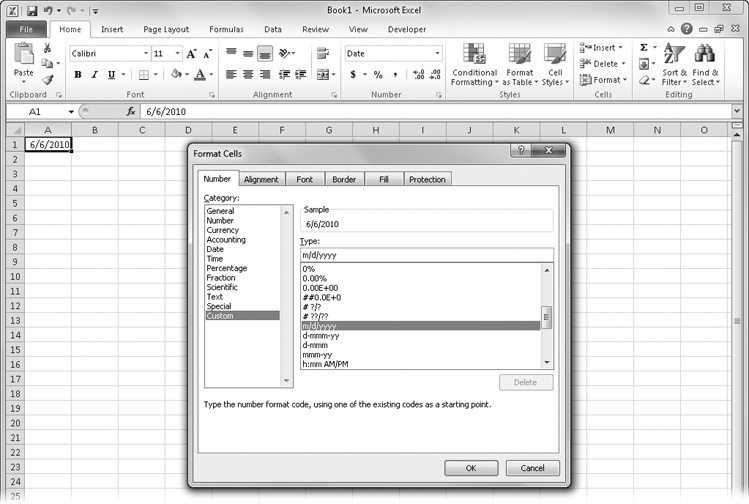
For example, to create a format that displays the date and time with the longest available format for day, month, and year, start by typing a date in a cell, and then select it. In the Custom category in the Format Cells dialog box, edit the format in the Type text box to read dddd, mmmm dd, yyyy – hh:mm AM/PM (including spaces and commas), and then click OK. Figure 9-42 shows the result.
Note
Saving the workbook saves your new formats, but to carry special formats from one workbook to another, you must copy and paste a cell with the Custom format. For easy access to special formats, consider saving them in one workbook.

You can create any number format using the codes in Table 9-1.
Table 9-1. Custom Format Symbols
Table 9-2 lists the built-in formats and indicates how these codes relate to the other categories on the Number tab. (This table does not list date and time codes, which are covered in Chapter 15.)
Table 9-2. Built-In Custom Format Codes
|
Category |
Custom Format Codes |
|---|---|
|
0 |
Digit |
|
General |
No specific format |
|
Number |
0 |
|
0.00 | |
|
#,##0 | |
|
#,##0.00 | |
|
#,##0_);(#,##0) | |
|
#,##0_);[Red](#,##0) | |
|
#,##0.00_);(#,##0.00) | |
|
#,##0.00_);[Red](#,##0.00) | |
|
Currency |
$#,##0_);($#,##0) |
|
$#,##0_);[Red]($#,##0) | |
|
$#,##0.00_);($#,##0.00) | |
|
$#,##0.00_);[Red]($#,##0.00) | |
|
Percentage |
0% |
|
0.00% | |
|
Scientific |
0.00E+00 |
|
##0.0E+0 | |
|
Fraction |
# ?/? |
|
# ??/?? | |
|
Date |
(See Chapter 15) |
|
Time |
(See Chapter 15) |
|
Text |
@ |
|
Accounting |
_($* #,##0_);_($* (#,##0);_($* “-”_);_(@_) |
|
_(* #,##0_);_(* (#,##0);_(* “-”_);_(@_) | |
|
_($* #,##0.00_);_($* (#,##0.00);_($* “-”??_);_(@_) | |
|
_(* #,##0.00_);_(* (#,##0.00);_(* “-”??_);_(@_) |
Creating Four-Part Formats Within each custom format definition, you can specify completely different formats for positive, negative, zero, and text values. You can create custom formats with as many as four parts, separating the portions by semicolons—positive number; negative number; zero; text. Figure 9-43 shows how three different formats are constructed using codes.

Note
You’ll find the Formatting Numbers.xlsx file with the other examples on the companion Web site. It contains many of the custom formatting code examples described in this section.
Among the built-in formats, only the Accounting formats use all four parts, as shown in Figure 9-43, which breaks down each part of the third Accounting format in Table 9-2. The following are some guidelines for creating multipart formats:
If your custom format includes only one part, Excel applies that format to positive, negative, and zero values.
If your custom format includes two parts, the first part applies to positive and zero values, and the second part applies only to negative values.
If your custom format has three parts, the third part controls the display of zero values.
The fourth and last element in a four-way format controls text-value formatting. Any formats with three or fewer elements have no effect on text entries.
Note
If you prefer, you can suppress the display of all zero values in a worksheet, including the displayed values of formulas with a zero result. Click the File tab, Options, and then click the Advanced category. In the Display Options For This Worksheet area, clear the Show A Zero In Cells That Have Zero Value check box.
Adding Color to Formats You can also use the Number formats to change the color of selected cell entries. For example, you might use color to distinguish categories of information or to make totals stand out. You can even create formats that assign different colors to specific numeric ranges so that, for example, all values greater than or less than a specified value appear in a different color.
Note
You can create codes that assign different colors based on the value in the cell, but an easier way is built into Excel: You can use the Conditional Formatting menu on the Home tab on the ribbon. For more information, see Formatting Conditionally on page 309.
To change the color of an entry, type the name of the new color in brackets in front of each segment of code. For example, if you want to apply a blue Currency format with two decimal places, edit the $#,##0.00_);($#,##0.00) format as follows:
[Blue]$#,##0.00_);($#,##0.00)
When you apply this format to a worksheet, positive and zero values appear in blue, and text and negative values appear as usual, in black. The following simple four-part format code displays positive values in blue, negative values in red, zero values in yellow, and text in green (with no additional number formatting specified).
[Blue];[Red];[Yellow];[Green]
You can specify the following color names in your formats: Black, Blue, Cyan, Green, Magenta, Red, White, and Yellow. You can also specify a color as COLORn, where n is a number in the range 1 through 16. Excel selects the corresponding color from your worksheet’s current 16-color palette.
Note
If you define colors that are not among your system’s repertoire of solids, Excel produces them by mixing dots from solid colors. Such blended colors, which are said to be dithered, work well for shading. But for text and lines, Excel always uses the nearest solid color rather than a dithered color.
TROUBLESHOOTING
Decimal points in my Currency formats don’t line up.
Sometimes when you use Currency formats with trailing characters, such as the French Canadian dollar (23.45 $), you want to use the GAAP practice of using currency symbols only at the top and bottom of a column of numbers. The numbers between should not display any currency symbols, so how do you make all the decimal points line up properly?
You can create a custom format code to apply to the noncurrency format numbers in the middle of the column. An underscore character (_) in the format code tells Excel to leave a space that is equal in width to the character that follows it. For example, the code _$ leaves a space equal to the width of the dollar sign. Thus, the following code does the trick for you:
#,##0.00 _$;[Red]#,##0.00 _$
Make sure you add a space between the zeros and the underscores to properly line the numbers up with the built-in French Canadian dollar format.
Using Custom Format Conditional Operators You can create custom formats that are variable. To do so, you can add a conditional operator to the first two parts of the standard four-part custom format. This, in effect, replaces the positive/negative formats with either/or formats. The third format becomes the default format for values that don’t match the other two conditions (the “else” format). You can use the conditional operators <, >, =, <=, >=, and <> with any number to define a format.
For example, suppose you are tracking accounts receivable balances. To display accounts with balances of more than $50,000 in blue, negative values in parentheses and in red, and all other values in the default color, create this format:
[Blue][>50000]$#,## 0.00_);[Red][<0]($#,##0.00);$#,##0.00_)
Using these conditional operators can also be a powerful aid if you need to scale numbers. For example, if your company produces a product that requires a few milliliters of a compound for each unit and you make thousands of units every day, you need to convert from milliliters to liters and kiloliters when you budget the use of this compound. Excel can make this conversion with the following numeric format:
[>999999]#,##0,,"kl";[>999]##,"L";#"ml"
The following table shows the effects of this format on various worksheet entries:
|
Entry |
Display |
|---|---|
|
72 |
72 ml |
|
7286957 |
7 kl |
|
7632 |
8 L |
As you can see, using a combination of conditional formats, the thousands separator, and text with spaces within quotation marks can improve both the readability and the effectiveness of your worksheet—and without increasing the number of formulas.
The Alignment group on the Home tab on the ribbon, shown in Figure 9-44, contains the most useful tools for positioning data within cells. For more precise control and additional options, click the dialog box launcher adjacent to the title of the Alignment group to display the Format Cells dialog box shown in Figure 9-45.
The Alignment tab in the Format Cells dialog box includes the following options:
Horizontal These options control the right or left alignment within the cell. The General option, the default for Horizontal alignment, right-aligns numeric values and left-aligns text values.
Vertical These options control the top-to-bottom position of cell contents within cells.
Text Control These three check boxes wrap text in cells, reduce the size of cell contents until they fit in the current cell width, and merge selected cells into one.
Text Direction The options in this drop-down list format individual cells for right-to-left languages. The default option is Context, which responds to the regional settings on your computer. (This feature is applicable only if support is available for right-to-left languages.)
Orientation These controls let you precisely specify the angle of text within a cell, from vertical to horizontal and anywhere in between.


The Align Left, Center, and Align Right buttons on the ribbon correspond to three of the options in the Horizontal drop-down list on the Alignment tab in the Format Cells dialog box: Left (Indent), Center, and Right (Indent). These options align the contents of the selected cells, overriding the default cell alignment. Figure 9-46 shows the Horizontal alignment options in action, all of which we’ll discuss in detail in the following sections.

Figure 9-46. Use the Horizontal alignment options to control the placement of text from left to right.

Indenting Cell Contents The Increase Indent button simultaneously applies left alignment to the selected cells and indents the contents by the width of one character. (One character width is approximately the width of the capital X in the Normal cell style.) Each click increments the amount of indentation by one. The adjacent Decrease Indent button does just the opposite, decreasing the indentation by one character width with each click.

In the Format Cells dialog box, the corresponding options are Left (Indent) and Right (Indent), shown in Figure 9-46. These are linked to the adjacent Indent control, whose displayed value is normally zero—the standard left-alignment setting. Each time you increase this value by one, the entry in the cell begins one character width to the right. For example, in Figure 9-46, row 2 is formatted with no left indent, row 3 with a left indent of 1, and row 4 with a left indent of 2. The maximum indent value you can use is 250.
Distributing Cell Contents Using the Distributed (Indent) option in the Horizontal drop-down list, you can position text fragments contained in a cell with equal spacing within the cell. For example, in Figure 9-46, we first merged cells A8:B8 into one cell, then typed the word Distributed three times in the merged cell, and then applied the Distributed (Indent) horizontal alignment. The result shows that Excel expanded the spaces between words in equal amounts to justify the contents within the cell.
Note
To learn about merging, see Merging and Unmerging Cells on page 365.
Centering Text Across Columns The Center Across Selection option in the Horizontal text alignment drop-down list centers text from one cell across all selected blank cells to the right or to the next cell in the selection that contains text. For example, in Figure 9-46, we applied the Center Across Selection format to cells A7:B7. The centered text is actually in cell A7.
Center Across Selection vs. Merge & Center
Although the result might look similar to that of the Merge & Center button on the Home tab, the Center Across Selection alignment option does not merge cells. When you use Center Across Selection, the text from the leftmost cell remains in its cell but is displayed centered across the entire selected range. Notice in the following figure that the selection shading shows that cells A1 and B1 are still two separate cells. The Merge & Center button creates a single cell in place of all the selected cells. Although Merge & Center merges rows and columns of cells, Center Across Selection works only on rows.

In the above figure, the text “Center Across Selection” actually spans two active cells, while the text “Merge & Center” is in a single cell that was created by selecting cells A2:B2 and clicking the Merge & Center button. Either method allows you to change column widths; the centering readjusts automatically. If you type anything in cell B1, the centered text “retreats” to cell A1; if you subsequently clear cell B1, the text is re-centered across the two cells until you clear the format from both cells. You cannot type anything in cell B2 because it essentially no longer exists after being merged with cell A2. For more information, see Merging and Unmerging Cells on page 365.
Filling Cells with Characters The Fill option in the Horizontal alignment drop-down list repeats your cell entry to fill the width of the column. For example, in Figure 9-46, cells A9:B9 contain the single word Fill and a space character, with the Fill alignment format applied. Only the first cell in the selected range needs to contain text. Excel repeats the text to fill the range. Like the other Format commands, the Fill option affects only the appearance, not the underlying contents, of the cell.
Caution
Because the Fill option affects numeric values as well as text, it can cause a number to look like something it isn’t. For example, if you apply the Fill option to a ten-character-wide cell that displays 3, the cell appears to contain the number 3333333333.

Wrapping Text in Cells If you type a label that’s too wide for the active cell, Excel extends the label past the cell border and into adjacent cells—provided those cells are empty. If you click the Wrap Text button on the Home tab (or the Wrap Text option on the Alignment tab in the Format Cells dialog box), Excel displays your label entirely within the active cell. To accommodate it, Excel increases the height of the row in which the cell is located and then wraps the text onto additional lines within the same cell. As shown in Figure 9-46, cell A10 contains a multiline label formatted with the Wrap Text option.
Justifying Text in Cells The Alignment tab in the Format Cells dialog box provides two justify options—one in the Horizontal drop-down list and one in the Vertical drop-down list. The Horizontal Justify option not only forces text in the active cell to align flush with the right margin, as shown in cell B10 in Figure 9-46, but also wraps text within the cell and adjusts the row height accordingly.
Note
Do not confuse the Horizontal Justify option with the Justify command (on the Fill menu in the Editing group on the Home tab), which redistributes a text entry into as many cells as necessary below the selected cell by dividing the text into separate chunks. For more information about the Justify command on the Fill menu, see Distributing Long Entries Using the Justify Command on page 236.
The Vertical Justify option performs essentially the same task as its Horizontal counterpart, except it adjusts cell entries relative to the top and bottom of the cell rather than the sides, as shown in cell E3 of Figure 9-47.
The Justify Distributed option becomes available only when you select one of the Distributed options in either the Horizontal drop-down list or the Vertical drop-down list. It combines the effect of the Justify option with that of the Distributed option not only by wrapping text in the cell and forcing it to align flush right but also by spacing the contents of the cell as evenly as possible within each wrapped line of text.


The Top Align, Middle Align, and Bottom Align buttons on the Home tab control the vertical placement of cell contents and fulfill most of your needs in this regard. The Vertical drop-down list on the Alignment tab in the Format Cells dialog box includes two additional alignment options—Justify and Distributed—which are similar to the corresponding Horizontal alignment options. Cells A3:C3 in Figure 9-47 show examples of the first three alignment options. As noted earlier, cell E3 shows the Justify option in action. We formatted cell D3, containing the percent signs, using the Distributed option.
The options in the Vertical drop-down list create the following effects:
Top, Center, and Bottom These options force cell contents to align to each respective location within a cell. The default vertical cell orientation in new worksheets is Bottom.
Justify This option expands the space between lines so that text entries align flush with the top and bottom of the cell.
Distributed This option spreads the contents of the cell evenly from top to bottom, making the spaces between lines as close to equal as possible.

Clicking the Orientation button in the Alignment group on the Home tab displays the menu shown in Figure 9-48, offering common orientation options.

The Orientation area on the Alignment tab in the Format Cells dialog box contains additional controls, letting you change the angle of cell contents to read at any angle from 90 degrees counterclockwise to 90 degrees clockwise.
A Cool Application of Angled Text
Many times the label at the top of a column is much wider than the data stored in it. You can use the Wrap Text option to make a multiple-word label narrower, but sometimes that’s not enough. Vertical text is an option, but it can be difficult to read and takes a lot of vertical space. Try using rotated text and cell borders:

Here’s how to do it:
Select the cells you want to format, and click the dialog box launcher in the Font group on the Home tab to display the Format Cells dialog box.
Click the Border tab, and apply vertical borders to the left, right, and middle of the range.
Click the Alignment tab, and use the Orientation controls to select the angle you want. (It’s usually best to select a positive angle from 30 to 60 degrees.)
In the Horizontal Text Alignment drop-down list, select Center, and then click OK. Excel rotates the left and right borders along with the text.
Drag down the bottom border of the row 1 header (the line between 1 and 2) to make it deep enough to accommodate the labels without wrapping.
Select all the active columns, and double-click any one of the lines between the selected column headers (for example, the line between the column letters C and D) to shrink all the columns to their smallest possible width.
Using the Angle Counterclockwise command on the Orientation button’s menu (in the Alignment group on the Home tab) rotates the text to +45 degrees for you, but because we wanted to apply borders and alignment options as well, using the Format Cells dialog box was a more efficient method.
Note
Interestingly, as you experiment with orientation, you won’t see a Horizontal option on the Orientation button’s menu. This means that you need to use either the Format Cells dialog box or the Undo command (Ctrl+Z) to restore cells to their default orientation.
Excel automatically adjusts the height of the row to accommodate vertical orientation unless you manually set the row height either before or after changing text orientation. Cell G3 in Figure 9-47 shows what happens when you click the tall, skinny Text button on the left side of the Orientation area. Although the button is labeled Text, you can also apply this “stacked letters” effect to numbers and formulas.
The angle controls let you rotate text to any point in a 180-degree arc. You can use either the Degrees box at the bottom or the large dial above it to adjust text rotation. To use the dial, click and drag the Text pointer to the angle you want; the number of degrees appears in the spinner below. You also can click the small up and down arrows in the Degrees box to increment the angle one degree at a time from horizontal (zero), or you can highlight the number displayed in the Degrees box and type a number from –90 through 90. Cells H3:K3 in Figure 9-47 show some examples of rotated text.
Note
For more about cell borders, see Customizing Borders on page 353. For more about row heights, see Changing Row Heights on page 364.
The Shrink To Fit check box on the Alignment tab in the Format Cells dialog box reduces the size of the font in the selected cell until the contents can be completely displayed in the cell. This is useful when you have a worksheet in which adjusting the column width to allow a particular cell entry to be visible has undesirable effects on the rest of the worksheet or where angled text, vertical text, and wrapped text aren’t feasible solutions. In Figure 9-49, we typed the same text in cells A1 and A2 (and increased the font size for readability) and applied the Shrink To Fit option to cell A2.

Figure 9-49. The Shrink To Fit alignment option reduces the font size until the cell contents fit within the cell.
The Shrink To Fit format is dynamic and readjusts if you change the column width, either increasing or decreasing the font size as needed. The assigned size of the font does not change; therefore, no matter how wide you make the column, the font will not expand beyond the assigned size.
The Shrink To Fit option can be a good way to solve a problem, but keep in mind that this option reduces the font to as small a size as necessary. If the cell is narrow enough and the cell contents long enough, the result might be too small to read.
The term font refers to a typeface (such as Calibri), along with its attributes (such as point size and color). The Font group on the Home tab on the ribbon, shown in Figure 9-50, is the easiest way to apply general font formatting to selected cells. Here are a few facts about the controls in the Font group:
The Font, Font Size, Underline, Borders, Fill Color, and Font Color buttons all include arrows to their right, which you can click to display a menu or gallery with additional options.
The appearance of the Font Color, Fill Color, and Borders buttons changes to reflect the last-used option. This lets you apply the same option again by clicking the button, without using the menu or gallery.
The Bold and Italic buttons are toggles; click once to apply the format, and click again to remove it.

For more extensive control over fonts, use the Font tab in the Format Cells dialog box. To specify a font, select the cell or range, click the dialog box launcher in the Font group, and then click the Font tab, shown in Figure 9-51.

Figure 9-51. On the Font tab you can assign fonts, character styles, sizes, colors, and effects to your cell entries.
The numbers in the Size list show the point sizes at which Excel can optimally print the selected font, but you can type any number in the text box at the top of the list—even fractional point sizes up to two decimal places. Unless you preset it, Excel adjusts the row height as needed to accommodate the largest point size in the row. The available font styles vary depending on the font you select in the Font list. Most fonts offer italic, bold, and bold italic styles. To reset the selected cells to the font and size defined as the Normal cell style, select the Normal Font check box.
Note
For more information about using cell styles, see Formatting with Cell Styles on page 303.
Tip
INSIDE OUT Automatic Font Color Isn’t Really Automatic
If you select Automatic (the default font color option) in the Color drop-down list (or use its equivalent in the Font group on the Home tab on the ribbon), Excel displays the contents of your cell in black. You might think that Automatic should select an appropriate color for text on the basis of the color you apply to the cell, but this isn’t the case. If, for example, you apply a black background to a cell, you might think the automatic font color would logically be white. This isn’t so; Automatic is always black unless you select another Window Font color in the Display Properties dialog box (accessed from Windows Control Panel). For more information about applying colors to cells, see Applying Colors and Patterns on page 357.

Borders and shading can be effective devices for defining areas in your worksheet or for drawing attention to important cells, and the Borders button in the Font group on the Home tab is the easiest way to apply them. Clicking this button applies the last-used border format and displays a thumbnail representation of it on the button. Click the arrow to the right of the button to display the menu shown in Figure 9-52.

Note
As does the image displayed on the button, the button name also reflects the last-used border format when you rest the pointer on the button to display a ScreenTip.
The most-often-used border options are represented on the Borders menu, but for more precise control, click the More Borders command on the menu to display the Border tab in the Format Cells dialog box, shown in Figure 9-53. (As always, the dialog box launcher next to the Font group opens the dialog box as well.) If you have more than one cell selected when you open the dialog box, the Border preview area includes tick marks in the middle and at the corners, as shown in Figure 9-53.

Note
A solid gray line in the preview area means that the format applies to some but not all of the selected cells.
An Angled Border Trick
Sometimes you might want to use that pesky cell that generally remains empty in the upper-left corner of a table. You can use an angled border to create dual-label corner cells (we expanded the formula bar in the following figure to show all the text in cell A3):

Here’s how to do it:
Select the cell you want to format, and type about 10 space characters. You can adjust this later (there are 20 spaces before the Exam # label in the example).
Type the label you want to correspond to the column labels across the top of the table.
Hold down the Alt key, and press Enter twice to create two line breaks in the cell.
Type the second label, which corresponds to the row labels down the left side of the table, and press Enter.
With the cell selected, click the More Borders command on the Borders menu.
Select a line style, and click the upper-left to lower-right angled border button.
Click the Alignment tab, select the Wrap Text check box, and then click OK.
You will probably need to fine-tune a bit by adjusting the column width and row height and by adding or removing space characters before the first label. In the example, we also selected cells B3:F3 and then clicked the Top Align button in the Alignment group on the Home tab so that all the labels line up across the top of the table.
Note
For more information about alignment, see Aligning Data in Cells on page 342. For more about entering line breaks and tabs in cells, see Formula-Bar Formatting on page 497.
To apply borders, you can click the preview area where you want the border to appear, or you can click the buttons located around the preview area. An additional preset button, Inside, becomes active only when you have more than one cell selected. If you click the Outline button, borders are applied only to the outside edge of the entire selection. The None preset removes all border formats from the selection.
Note
Borders often make a greater visual impact on your screen when you remove worksheet gridlines. Click the View tab on the ribbon, and clear the Gridlines check box in the Show/Hide group to remove gridlines from your worksheet. For more information about gridlines, see Controlling Other Elements of the Excel 2010 Interface on page 103.
The default, or Automatic, color for borders is black. To select a line style, click the type of line you want to use in the Line area, and then click any of the buttons in the Border area or click the preview box directly to apply that style in the selected location. (The first finely dotted line in the Style area is a solid hairline when printed.) To remove a border, click the corresponding button—or the line in the preview window—without selecting another style.
By using the commands in the Draw Borders group at the bottom of the Borders menu (shown in Figure 9-52), you can create complex borders quickly and easily. When you click Draw Border, you enter “border-drawing mode,” which persists until you click Draw Border again or press Esc. After you activate this mode, you can drag to create lines and boxes along cell gridlines, as shown in Figure 9-54. If you click Draw Border Grid, not only are borders drawn along the boundaries of the selected cells, but they’re also drawn along all the gridlines in the selection rectangle, as shown at the bottom of Figure 9-54.
If you make selections in the Line Color and Line Style galleries at the bottom of the Borders menu prior to using either Draw Border command, the borders you draw reflect your color and style selections. Clicking Erase Border predictably activates the opposite of border-drawing mode: “border-erasing mode.” Dragging while in erase mode removes all borders within the selection rectangle.


The Fill Color button in the Font group on the Home tab offers colors you can apply to selected cells. Click the button’s arrow to display the options shown in Figure 9-55.

If you want to do more than just fill cells with color, the Fill tab in the Format Cells dialog box provides additional control. (Click the dialog box launcher in the Font group on the ribbon to display the Format Cells dialog box.) The main feature of the Fill tab is a palette of colors, mimicking the palette available on the ribbon. A feature not available on the ribbon is the Pattern Style drop-down palette, shown in Figure 9-56. You use this palette to select a pattern for selected cells and the Pattern Color drop-down palette above it to choose a color.

Follow these guidelines when using the Fill tab:
The Background Color area controls the background of selected cells. When you choose a color and do not select any pattern, Excel applies a solid colored background.
To return the background color to its default state, click No Color.
If you pick a background color and then select a pattern style, the pattern is overlaid on the solid background. For example, if you select red from the Background Color area and then click one of the dot patterns, the result is a cell that has a red background and black dots.
The Pattern Color options control the color of the pattern, not the cell. For example, if you leave Background Color set to No Color and select a red for Pattern Color and any dot pattern for Pattern Style, the cell is displayed with a white background with red dots.
Note
When selecting colors for cell backgrounds, select one on which you can easily read any text or numbers in the cell. For example, yellow is the most visible background color you can choose to complement black text, which is why you see this combination on road signs. A dark blue background with black text—that’s not so good.
The More Colors button on the Fill tab displays the Colors dialog box shown in Figure 9-57, where you can select colors that are not otherwise represented on the color palettes. The Standard tab in the Colors dialog box displays a stylized color wheel using the current theme colors, most of which are already available on the palettes. The Custom tab shown in Figure 9-57 lets you pinpoint colors, use specific color values, and switch between the default RGB (red, green, blue) color model or HSL, a color model defined by hue, saturation, and luminosity values instead of RGB color values.
The Fill Effects button on the Fill tab in the Format Cells dialog box opens up another world of possibility, offering gradient fills you can apply to cells. Clicking this button displays the Fill Effects dialog box shown in Figure 9-58. You can select different colors and shading styles, but this version of the Fill Effects dialog box offers only two-color effects. The One Color and Preset options are not available. Note that Fill Effects gradient fills are static, unlike data bars, which are conditional gradient fills that respond to cell values and interact with adjacent cells by applying proportional amounts of fill to each cell.
Note
For more about gradients, see Filling an Area with a Color Gradient on page 702. For more about data bars, see Formatting Conditionally on page 309.

Figure 9-57. Click the More Colors button on the Fill tab in the Format Cells dialog box to select the colors you need.

Figure 9-58. Click the Fill Effects button on the Fill tab in the Format Cells dialog box to use gradient fills in cells.

Adding background images to worksheets is easy. Click the Page Layout tab on the ribbon, and click the Background button. A standard Windows file-management dialog box appears, from which you can open most types of image files, located anywhere on your computer or network. Excel then applies the graphic image to the background of the active worksheet, as shown in Figure 9-59.
Here are some tips for working with background images:
The example in Figure 9-59 is a cover sheet for a large workbook; be careful when using backgrounds behind data. It can be difficult to read cell entries with the wrong background applied.
You might want to turn off the display of gridlines, as shown in Figure 9-59. To do so, clear the Gridlines View check box, which is also located on the Page Layout tab.
If you don’t like the way the background looks with your data, click the Background button again, whose name changes to Delete Background when a background is present.
The graphic image is tiled in the background of your worksheet, which means the image is repeated as necessary to fill the worksheet.
Cells to which you have assigned a color or pattern override the graphic background.
Backgrounds are preserved when you save the workbook as a Web page.
Note
For more information about saving workbooks as Web pages, see Chapter 26.
The primary methods you use to control the size of cells are adjusting the row height and changing the column width. In addition, you can adjust the size of cells by merging several cells into one or by unmerging previously merged cells. The Format menu, located in the Cells group on the Home tab, is the central command location for cell sizing, as shown in Figure 9-60.

Figure 9-60. You can use the Cell Size commands on the Format menu to manage row height and column width.
Here are the options you can use:
Column Width and Row Height These two commands display a dialog box where you can type a different value to be applied to selected cells. Column width is limited to 255, and row height can be up to 409. The default column width for Excel is 8.43 characters; however, this does not mean each cell in your worksheet can display 8.43 characters. Because Excel uses proportionally spaced fonts (such as Arial) as well as fixed-pitch fonts (such as Courier), different characters can take up different amounts of space. A default-width column, for example, can display about eight numerals in most 10-point fixed-pitch fonts.
AutoFit Row Height This command adjusts the row height in selected cells by adjusting them to accommodate the tallest item in the row. (Row height is usually self-adjusting based on font size.)
AutoFit Column Width This command adjusts column widths in selected cells by adjusting them to accommodate the widest entry in the column.
Default Width This command displays a dialog box where you can change the starting column width for all selected worksheets in the current workbook. This has no effect on columns whose width you have previously specified.
If the standard column width isn’t enough to display the complete contents of a cell, one of the following will occur:
To change column widths using the mouse, drag the lines between column headings. As you drag, the width of the column and the number of pixels appear in a ScreenTip, as shown in Figure 9-61. This figure also illustrates how to change the width of multiple columns at the same time: Drag to select column headings; alternatively, hold down Ctrl, and click headings to select nonadjacent columns. Then, when you drag the line to the right of any selected column, all the selected column widths change simultaneously.

Figure 9-61. The cursor looks like a double-headed arrow when you adjust column width or row height with the mouse.
Note
Depending on the font you are using, characters that appear to fit within a column on your screen might not fit when you print the worksheet. You can preview your output before printing by pressing Ctrl+P to display the Print screen in Backstage View, where you can see an image of the worksheet as it will look when printed. For information about print preview, see Chapter 11.
The height of a row always changes dynamically to accommodate the largest font used in that row. Thus, you don’t usually need to worry about characters being too tall to fit in a row. Adjusting row height is the same as adjusting column width—just drag one of the lines between row headings.
To restore the default height of one or more rows, select any cell in those rows, and click AutoFit Row Height on the Format menu on the Home tab. Unlike column width, you cannot define a standard row height. The AutoFit command serves the same function, returning empty rows to the standard height needed to accommodate the default font and fitting row heights to accommodate the tallest entry. When you create or edit a multiline text entry using the Wrap Text button or the Justify option on the Alignment tab in the Format Cells dialog box, Excel automatically adjusts the row height to accommodate it.

The spreadsheet grid is arguably the most versatile type of document, and the ability to merge cells makes it all the more versatile. Select the cells you want to merge, and click the arrow to the right of the Merge & Center button in the Alignment group on the Home tab to display the menu shown in Figure 9-62.
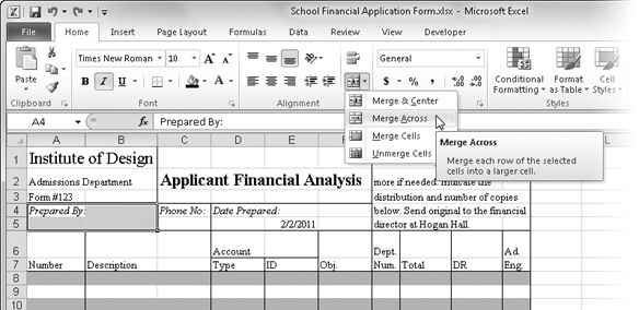
Caution
When you merge several cells that contain data, only the data in the uppermost, leftmost cell is preserved. Excel overwrites data in subsidiary cells. Copy any data you need to another location before merging.
When you merge cells, you end up with a single cell that comprises the original cells. If in the worksheet shown in Figure 9-63, we were to select cells A4:B5 and click the Merge Across command, the result would be two merged cells, A4 and A5, each spanning two columns. Here are the differences between the Merge & Center commands:
Merge & Center This command consolidates all selected cells—both rows and columns—into one big cell and centers the contents across the newly merged cell.
Merge Across This command consolidates each row of selected cells into one wide cell per row.
Merge Cells This command consolidates all selected cells into one big cell, but it does not center the contents.
Unmerge Cells This command returns a merged cell to its original component cells and places its contents in the upper-leftmost cell. Clicking the Merge & Center button (not the Merge & Center command) when a merged cell is selected has the same effect, like a toggle “turning off” the merge.

Figure 9-63. Most of the cells in the top five rows of this worksheet, and a couple in the sixth row, are merged in various combinations.
Figure 9-63 shows the same worksheet shown in Figure 9-62 after merging cells A1:B3, C1:F3, G1:J5, A4:B4, A5:B5, D4:F4, D5:F5, and D6:E6. We had to shuffle some of the text, before merging so that we wouldn’t lose it to the merging process. For example, the text in the original range G1:J5 was unevenly spaced because of the different row heights needed to accommodate the text in cells A1 and C2. To eliminate this problem, we used the Merge Cells command on the range A1:B3, we used the Merge & Center command on the ranges C1:F3 and G1:J5, and then we reentered the text.
Note
You’ll find the School Financial Application Form.xlsx file with the other examples on the companion Web site.
When you merge cells, the new big cell uses the address of the cell in the upper-left corner, as shown in Figure 9-63. Cell A1 is selected, as you can see in the Name box. (In the figure, we also expanded the formula bar to show the three rows of text in the merged cell.) The headings for rows 1, 2, and 3 and columns A and B are highlighted, which would ordinarily indicate that the range A1:B3 is selected. For all practical purposes, however, cells A2:A3 and B1:B3 no longer exist. The other merged cells, or the subsidiary cells, act like blank cells when referred to in formulas and return zero (or an error value, depending on the type of formula).
Note
In Figure 9-63, the information in the formula bar is on three lines. To enter line breaks within a cell, press Alt+Enter. For more information, see Formula-Bar Formatting on page 497.
Merging cells obviously has interesting implications, considering that it seems to violate the grid—one of the defining attributes of spreadsheet design. That’s not as bad as it sounds, but keep in mind these tips:
If you select a range to merge and any single cell contains text, a value, or a formula, the contents are relocated to the new big cell.
If you select a range of cells to merge and more than one cell contains text or values, only the contents of the uppermost, leftmost cell are relocated to the new big cell. Contents of subsidiary cells are deleted; therefore, if you want to preserve data in subsidiary cells, make sure you add it to the upper-left cell or relocate it.
Formulas adjust automatically. A formula that refers to a subsidiary cell in a merged range changes to refer to the address of the new big cell. If a merged range of cells contains a formula, relative references adjust. For more about references, see Using Cell References in Formulas on page 468.
You can copy, delete, cut and paste, or click and drag big cells as you would any other cell. When you copy or move a big cell, it replaces the same number of cells at the destination. The original location of a cut or deleted big cell returns to individual cells.
You can drag the fill handle of a big cell as you can drag the fill handle of regular cells. When you do so, the big cell is replicated, in both size and content, replacing all regular cells in its path. For more about using the fill handle, see Filling and Creating Data Series on page 229.
If you merge cells containing border formatting other than along any outer edge of the selected range, border formats are erased.